
- Dynamic System Modeling: Formulate linear time-invariant (LTI) differential equations, Laplace transfer functions, and multi-input multi-output (MIMO) state-space state matrices.
- Stability & Robustness Metrics: Evaluate asymptotic stability using the Routh-Hurwitz criterion, Root Locus trajectories, and Bode frequency response gain/phase margins.
- Advanced Control Architectures: Synthesize closed-loop PID gains with anti-windup, state-feedback pole placement via Ackermann's formula, and Model Predictive Control (MPC) with actuator constraints.
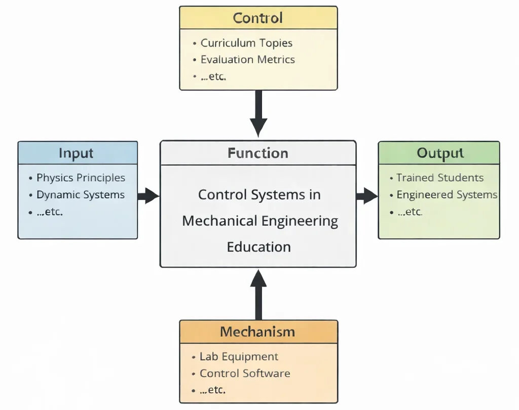
- Inputs (Left): Multi-body plant dynamics, reference trajectory profiles, sensor noise spectra, external load disturbances, and actuator bandwidth constraints.
- Controls (Top): Washington Accord/EUR-ACE engineering benchmarks, ISO 13849 safety of machinery standards, IEC 61131-3 PLC programming criteria, and gain/phase margin design specifications.
- Mechanisms (Bottom): MATLAB/Simulink simulation suites, hardware-in-the-loop (HIL) microcontrollers, real-time operating systems (RTOS), optical encoders, and servo-hydraulic testbeds.
- Outputs (Right): Robust closed-loop controller firmware, certified fail-safe motion actuators, verified stable step responses, and practice-ready control systems engineers.
Mechanical & Control Engineering Curriculum Cluster
Select any foundational pillar below to explore related modules across the PREP4UNI.ONLINE Mechanical Engineering series:
Mechanical Engineering
Supplies the physical differential plant equations that control architectures stabilize and optimize.
Automotive Engineering
Executes active yaw moment control, electronic torque vectoring, and autonomous lane-centering control.
Biomechanical Engineering
Models closed-loop physiological homeostatic loops, insulin pump regulators, and neural motor feedback.
Control Systems in Mechanical Engineering
PID loop tuning, state-space estimators, frequency response Bode analysis, and optimal dynamic stability.
Fluid Mechanics and Hydraulics
Regulates electro-hydraulic proportional valves, flow control manifolds, and surge-tank pressure balances.
Manufacturing and Production Engineering
Oversees multi-axis CNC interpolation, PLC ladder logic sequences, and automated quality scrap tracking.
Mechanical Design and CAD
Integrates motor housings, encoder wiring harnesses, and structural sensor brackets into digital master assemblies.
Nanotechnology and Advanced Materials
Utilizes shape memory alloys, electrostrictive ceramics, and magnetorheological fluid adaptive dampers.
Robotics and Automation in Mechanical Engineering
Applies computed-torque algorithms and inverse kinematic control to 6-DOF industrial robot arms.
Solid Mechanics: Stress, Strain & Structural Analysis
Compensates for link elastic deflections and structural compliance during high-speed precision positioning.
Thermodynamics and Heat Transfer
Executes closed-loop PID control over heat exchanger bypass valves, chillers, and furnace heating zones.
Vibrations and Acoustics
Drives active anti-phase noise cancellation and electromagnetic dampers to eliminate resonance.

Deep Technical Foundations: Analytical Control Theory & Dynamics
Control systems engineering converts mechanical dynamics into tractable mathematical architectures. Mastering the field requires proficiency across Laplace-domain transfer functions, time-domain state-space formulations, and frequency-domain stability criteria.
1. Second-Order System Dynamics & Step Response Characteristics
A prototypical mechanical mass-spring-damper plant driven by control force u(t) satisfies the linear differential equation mẍ + cẋ + kx = u(t). Taking Laplace transforms with zero initial conditions yields the standard canonical second-order closed-loop transfer function:
$$T(s) = \frac{X(s)}{R(s)} = \frac{\omega_n^2}{s^2 + 2\zeta\omega_n s + \omega_n^2}$$where ωn = √(k/m) is the undamped natural frequency in rad/s, and ζ = c / (2√(km)) is the dimensionless damping ratio. For an underdamped system (0 < ζ < 1), the closed-loop poles reside at complex conjugate locations s = −ζωn ± jωd, where ωd = ωn√(1 − ζ2) is the damped natural frequency. The transient step response exhibits peak percentage overshoot (%Mp), peak time (tp), and 2% settling time (ts) governed by:
$$\%M_p = \exp\left( -\frac{\zeta\pi}{\sqrt{1 - \zeta^2}} \right) \times 100\%, \qquad t_p = \frac{\pi}{\omega_d} = \frac{\pi}{\omega_n\sqrt{1 - \zeta^2}}, \qquad t_s \approx \frac{4}{\zeta\omega_n}$$2. State-Space Representation & Pole Placement
For complex multi-degree-of-freedom mechanical systems, dynamics are represented in continuous-time first-order vector-matrix state-space form:
$$\mathbf{\dot{x}}(t) = \mathbf{A}\mathbf{x}(t) + \mathbf{B}\mathbf{u}(t), \qquad \mathbf{y}(t) = \mathbf{C}\mathbf{x}(t) + \mathbf{D}\mathbf{u}(t)$$where the state vector x represents physical coordinates (displacements and velocities), u is the control input vector, and y is the measurement output vector. The system is completely controllable if and only if the controllability matrix has full rank n:
$$\text{rank}(\mathcal{C}) = \text{rank}\left( \begin{bmatrix} \mathbf{B} & \mathbf{AB} & \mathbf{A}^2\mathbf{B} & \dots & \mathbf{A}^{n-1}\mathbf{B} \end{bmatrix} \right) = n$$Under full state-feedback control u(t) = −Kx(t) + r(t), the closed-loop system matrix becomes (A − BK). Controller gain matrix K is uniquely calculated via Ackermann's formula to place eigenvalues at desired pole locations defined by the target characteristic polynomial αc(s):
$$\mathbf{K} = \begin{bmatrix} 0 & 0 & \dots & 1 \end{bmatrix} \mathcal{C}^{-1} \alpha_c(\mathbf{A})$$3. Frequency Response & Robust Stability Margins
Substituting s = jω into the open-loop transfer function L(s) = Gc(s)Gp(s) yields the frequency response function L(jω) = |L(jω)|ej∠L(jω). Stability robustness is quantified by the Gain Margin (GM) and Phase Margin (PM):
$$\text{Gain Crossover Frequency } \omega_{gc}: \ |L(j\omega_{gc})| = 1 \ (0\text{ dB}) \quad \Rightarrow \quad \text{PM} = 180^\circ + \angle L(j\omega_{gc})$$ $$\text{Phase Crossover Frequency } \omega_{pc}: \ \angle L(j\omega_{pc}) = -180^\circ \quad \Rightarrow \quad \text{GM} = \frac{1}{|L(j\omega_{pc})|} \Rightarrow -20\log_{10}|L(j\omega_{pc})|\text{ dB}$$For robust closed-loop stability under plant parameter variations and high-frequency sensor noise, engineering guidelines specify minimum margins of PM ≥ 45° to 60° and GM ≥ 6 dB.
Contemporary Computational Paradigms in Control Systems
Industrial mechanical automation has moved beyond single-loop analog controllers to unified digital networks integrating physics-based estimators, neural approximations, and predictive horizon solvers:
Model Predictive Control (MPC) with QP Solvers
MPC executes real-time dynamic optimization over a finite prediction horizon Np, solving a Quadratic Programming (QP) cost function subject to hard actuator saturation limits (|u| ≤ umax) and slew rate limits (|u̇| ≤ u̇max). It provides superior multivariable coordination in autonomous driving and gas turbine control.
Physics-Informed Neural Networks (PINNs) in Adaptive Control
PINNs identify non-linear mechanical friction, aerodynamic drag, and thermal dissipation models in real time by embedding Newton-Euler differential equations into the loss formulation. This allows self-tuning controllers to adapt feedforward gains without destabilizing closed-loop operations.
Digital Twins & Kalman Filter Telemetry
Cyber-physical digital twins run Extended Kalman Filters (EKF) alongside real-time factory machinery. By fusing sparse encoder and accelerometer telemetry with full-order physical models, the digital twin estimates unmeasurable internal motor temperatures, gear backlash, and dynamic torsional deflections.
Systems Engineering Trade-off Matrix
Control systems design requires balancing competing operational goals: fast rise times elevate overshoot, while aggressive disturbance rejection amplifies high-frequency sensor noise.
| Control Strategy / Architecture | Primary Engineering Advantage | Bottlenecks & Failure Modes | Mitigation & Control Strategy |
|---|---|---|---|
| High Proportional Gain (Kp ≫ 1) | Dramatically reduces rise time (tr); increases disturbance rejection stiffness; reduces steady-state error under static load. | Drives closed-loop poles toward imaginary axis; induces severe transient overshoot; causes physical actuator torque saturation and chattering. | Add derivative feedback (Kd) or a lead compensator to inject phase lead; implement input saturation limiters in controller software. |
| Integral Action Accumulation (Ki / s) | Eliminates steady-state error (ess → 0) under step reference inputs and constant external torque disturbances (Type 1 system). | Introduces −90° phase lag; degrades phase margin; triggers integrator windup during actuator saturation, causing delayed recovery. | Implement anti-windup clamping (back-calculation or conditional integration); clamp integrator state when actuator reaches physical saturation. |
| Pure Derivative Feedback (Kd · s) | Provides predictive phase lead; dampens high-frequency resonant oscillations; shortens settling time (ts). | Acts as high-pass filter, infinitely amplifying high-frequency sensor noise and quantization jitter; damages mechanical gear teeth. | Cascade derivative term with a low-pass filter: D(s) = [Kds] / [1 + s/(Nωc)], setting filter coefficient N ≈ 8 to 20. |
| Model Predictive Control (MPC) | Explicitly handles multivariable MIMO interactions; enforces strict physical constraints on voltage, pressure, and displacement. | Computationally intensive; requires real-time convex QP solvers; software failure occurs if optimization does not converge within cycle time. | Deploy explicit offline MPC look-up tables for fast embedded microcontrollers; implement fall-back classical PID supervisory watchdogs. |
Cross-Sector Industrial Case Studies
Aerospace Fly-by-Wire Flight Control
Modern commercial airliners operate with statically relaxed longitudinal stability to minimize trim drag. Triply-redundant digital flight controllers process pitot pressure, inertial gyros, and pilot sidestick inputs at 100 Hz, commanding electro-hydraulic actuators on ailerons and elevators to enforce flight envelope protection.
Automotive Active Suspension & ESC
Electronic Stability Control (ESC) systems evaluate vehicle yaw-rate sensors against steering angle inputs. When cornering on icy asphalt induces oversteer, differential braking control loops apply precise brake pulses to outer wheels within 15 milliseconds, generating counter-yaw moments that prevent spin-out.
High-Speed 5-Axis CNC Machining Centers
Milling aerospace titanium blisks requires maintaining sub-5-micron path tracking at feedrates of 15 m/min. Cascaded control architectures pair 16-kHz current loops with 4-kHz velocity loops and optical linear encoder feedback, utilizing jerk-limited trajectory profiles to eliminate structural chatter.
Wind Turbine Blade Pitch Control
To protect 15-MW offshore wind turbines in turbulent storm gusts, independent pitch control (IPC) systems use hydraulic cylinders or brushless AC servo motors to feather each blade individually once per revolution, attenuating asymmetric aerodynamic fatigue loads across the main bearing.
Interactive Simulation: Closed-Loop PID Step Response Engine
Evaluate real-time closed-loop transient dynamics, peak overshoot, rise time, and settling time for a continuous second-order mechanical system (mẍ + cẋ + kx = u) regulated by an interactive PID feedback controller.
Closed-Loop PID Control & Step Response Engine
STATUS: ACTIVE SOLVERFrequently Asked Questions: Control Theory & Industrial Systems
1. What distinguishes modern state-space control from classical transfer-function control?
2. How does the Routh-Hurwitz criterion determine absolute stability without calculating roots?
3. Why does derivative feedback require low-pass filtering in practical microcontroller deployments?
4. What is integrator windup, and how do anti-windup clamping algorithms mitigate it?
5. How does the Phase Margin correlate directly with closed-loop damping ratio?
6. What is the fundamental difference between feedforward and feedback control?
7. How do Root Locus trajectories assist in feedback gain selection?
8. How does digital discretization (Z-transform) alter continuous-time stability?
Student Practice & Accreditation Assessment Modules
Section 1: Interactive Knowledge Self-Assessment
Q1: Formulate why adding an open-loop pole shifts root locus branches to the right, degrading stability.
Q2: Differentiate between Type 0, Type 1, and Type 2 control systems regarding steady-state tracking error.
- Type 0: Zero integrators; exhibits finite steady-state error ess = 1/(1+Kp) to step inputs, and infinite error to ramps.
- Type 1: One integrator; achieves zero error (ess = 0) to step inputs, but finite error ess = 1/Kv to ramp inputs.
- Type 2: Two integrators; achieves zero error to step and ramp inputs, and finite error ess = 1/Ka to parabolic acceleration inputs.
Q3: Why does a lead compensator improve transient response, while a lag compensator improves steady-state accuracy?
Q4: How does state observability determine whether an unmeasured state can be reconstructed using a Luenberger observer?
Q5: Why do non-minimum phase zeros (zeros in the right-half plane) impose fundamental limitations on feedback control?
Q6: What causes limit-cycle oscillations in feedback loops with mechanical backlash and friction?
Q7: How does cascade control improve disturbance rejection compared to a single feedback loop?
Q8: Formulate the Nyquist Stability Criterion for an open-loop transfer function with unstable poles.
Section 2: Analytical & Scenario-Based Case Studies
Scenario: A 150-kW industrial electric annealing furnace experienced severe temperature overshoot (+85°C above target) and thermal stress cracks during batch startup, despite being regulated by a tuned industrial PID controller.
Engineering Evaluation:
1. Actuator Limits: The electric thyristor heaters saturated at 100% duty cycle for 25 minutes while heating the cold furnace from ambient to 650°C.
2. Windup Dynamics: Because error e(t) = Tset − T(t) remained positive, the integral term continued to accumulate:
$$u_I(t) = K_i \int_0^t e(\tau) d\tau \to \text{Max Integer Overflow}$$
When the furnace reached 650°C, the controller could not reduce heating power because the saturated integral state required 12 minutes of negative error to discharge, causing deep temperature overshoot.
Corrective Engineering Action: Implement a back-calculation anti-windup algorithm. When actuator saturation is detected, the difference between saturated actuator output and calculated controller demand is fed back through an anti-windup gain 1/Tt to discharge the integrator dynamically.
Scenario: A six-axis articulated industrial robot arm exhibited audible acoustic buzzing and high-frequency torque oscillations (85 Hz) when holding static payload positions.
Engineering Evaluation:
The optical encoder had a low resolution of 1024 pulses per revolution (PPR). At static hold, the position signal oscillated between adjacent quantization counts (±1 LSB). The derivative control term calculated numerical differences:
$$\frac{de(t)}{dt} \approx \frac{e[k] - e[k-1]}{T_s}$$
With sample time Ts = 0.001 s, this discrete jump produced derivative force spikes exceeding 35 N·m, driving the motor current amplifier into continuous chattering.
Corrective Engineering Action: Replace raw finite-difference derivative calculation with a second-order Savitzky-Golay polynomial filter or a Kalman state estimator. Upgrade the optical joint feedback to a 20-bit absolute magnetic encoder (1,048,576 counts/rev) to minimize quantization steps.
Scenario: A deepwater subsea remotely operated vehicle (ROV) robotic arm experienced uncontrollable limit-cycle oscillations whenever grasping structural wellhead equipment over an umbilical cable link.
Engineering Evaluation:
The 3000-meter fiber-optic tether and surface tele-operation software introduced a round-trip communication latency τ = 65 ms. In the frequency domain, transport delay introduces pure phase lag without magnitude attenuation:
$$\phi_{\text{delay}}(\omega) = -\omega \tau \text{ rad}$$
At the crossover frequency ωgc = 24 rad/s, the delay injected −89.4° of phase lag, eroding the open-loop phase margin from +48° to −41.4° and driving the closed-loop poles into the right-half plane.
Corrective Engineering Action: Restructure the control architecture by embedding a local high-bandwidth closed-loop controller on the subsea vehicle, feeding supervisory setpoints via a Smith Predictor time-delay compensator to preserve phase margin.
Scenario: An Earth-observation imaging satellite developed jitter and loss of attitude lock whenever its reaction wheel attitude control loop commanded rapid slew maneuvers.
Engineering Evaluation:
The closed-loop attitude controller was tuned with a bandwidth of ωBW = 12 rad/s (1.91 Hz). The flexible solar array appendages possessed a fundamental structural torsional vibration mode at ωstruct = 1.85 Hz with low damping (ζ = 0.005). The reaction wheel's control energy excited this resonant appendage mode, establishing an unstable control-structure interaction (spillover).
Corrective Engineering Action: Insert a digital notch filter into the control loop centered at 1.85 Hz:
$$G_{\text{notch}}(s) = \frac{s^2 + \omega_0^2}{s^2 + 2\zeta_n \omega_0 s + \omega_0^2}$$
attenuating controller gain by 28 dB at the structural resonance frequency to prevent excitation.
Scenario: When steam turbine load surged suddenly, an industrial power plant boiler drum water level controller commanded feedwater valves open, but the measured water level initially dropped sharply, tripping emergency shutdown sensors.
Engineering Evaluation:
Boiler drum dynamics exhibit a non-minimum phase phenomenon known as "shrink and swell." Cold feedwater injected into boiling water condenses steam bubbles below the surface, causing the liquid level to shrink temporarily before rising. The transfer function contains a zero in the right-half plane:
$$G(s) = \frac{K(-T_a s + 1)}{s(T_1 s + 1)}$$
A fast feedback controller reacted to the initial level drop by forcing valves further open, amplifying bubble condensation and destabilizing the drum.
Corrective Engineering Action: Implement a three-element feedforward boiler control architecture that measures steam mass flow rate directly, injecting feedforward commands proportional to steam demand to bypass non-minimum phase level dynamics.
Scenario: A heavy coastal surveillance radar antenna developed sustained 4.5-Hz azimuth hunting oscillations when attempting to lock onto stationary nautical targets.
Engineering Evaluation:
Mechanical wear in the main bull gear introduced mechanical backlash of θb = 0.35°. When the high-gain PID controller drove the dish toward the setpoint, the antenna entered the gear clearance deadband, uncoupling drive motor inertia from antenna load inertia. The controller overcompensated for the zero-resistance zone, creating a classic non-linear limit cycle.
Corrective Engineering Action: Install a dual-motor electrical anti-backlash drive system. Two pinion motors are driven in opposite torque directions (bi-directional torque preloading), keeping gear teeth permanently engaged against opposing faces to eliminate deadbands.
Scenario: Full Authority Digital Engine Control (FADEC) development testing on a two-spool turbofan engine showed compressor surge when the fuel metering valve and variable stator vanes operated simultaneously.
Engineering Evaluation:
Engineers had designed two independent single-input single-output (SISO) PID loops for fuel flow (controlling high-pressure core speed N2) and variable stator vane angle (controlling low-pressure fan speed N1). Strong thermodynamic aerodynamic cross-coupling between the spools was ignored. The off-diagonal transfer functions induced cross-talk:
$$\mathbf{G}(s) = \begin{bmatrix} G_{11}(s) & G_{12}(s) \\ G_{21}(s) & G_{22}(s) \end{bmatrix}$$
When one loop corrected for an airflow perturbation, it disturbed the other, causing aerodynamic surge.
Corrective Engineering Action: Replace independent SISO controllers with a multivariable H∞ robust controller or Model Predictive Control (MPC) based on a coupled 2×2 state-space model, decoupling spool dynamics and enforcing compressor surge margins.
Section 3: Step-by-Step Quantitative Worked Examples
Problem Statement: A unity feedback position control system has an open-loop plant transfer function:
$$G(s) = \frac{20}{s(s + 5)}$$
Calculate:
(a) The closed-loop transfer function T(s) = Y(s)/R(s).
(b) The undamped natural frequency (ωn) in rad/s and damping ratio (ζ).
(c) The closed-loop pole locations in the complex s-plane.
(d) The peak percentage overshoot (%Mp) and 2% settling time (ts).
Problem Statement: An industrial thermal process plant regulated under unity feedback has forward open-loop transfer function:
$$G(s) = \frac{4}{3s + 1}$$
Calculate:
(a) The static position error constant (Kp) and steady-state tracking error (ess,step) for a unit step input R(s) = 1/s.
(b) The steady-state tracking error (ess,ramp) for a unit ramp input R(s) = 1/s2.
(c) Sizing an integral controller Gc(s) = Ki / s to eliminate steady-state error to step inputs.
Problem Statement: A DC servo motor velocity plant is modeled by the first-order transfer function:
$$G_p(s) = \frac{1}{s + 2}$$
A proportional controller with gain Kp = 12.0 is implemented in a unity feedback loop. Calculate:
(a) The closed-loop characteristic equation and pole location.
(b) The closed-loop system time constant (τ).
(c) The closed-loop −3 dB bandwidth frequency (ωBW) in rad/s.
(d) Compare the uncompensated plant time constant with the compensated closed-loop time constant.
Problem Statement: A third-order feedback system has closed-loop characteristic polynomial:
$$q(s) = s^3 + 6s^2 + 11s + K = 0$$
where K is an adjustable controller gain.
(a) Construct the Routh array in terms of parameter K.
(b) Determine the range of gain K for which the closed-loop system is strictly stable.
(c) Determine the critical gain value (Kcrit) that induces marginal stability and compute the resulting frequency of sustained oscillation (ωosc).
When K = 66, the s1 row becomes zero (b1 = 0).
Form auxiliary equation from the s2 row:
$$6s^2 + K = 0 \Rightarrow 6s^2 + 66 = 0 \Rightarrow s^2 = -11$$ $$s = \pm j\sqrt{11} \approx \pm j 3.3166 \text{ rad/s}$$ $$\omega_{\text{osc}} = \sqrt{11} \approx 3.32 \text{ rad/s} \quad \left( f_{\text{osc}} = \frac{3.3166}{2\pi} \approx 0.528 \text{ Hz} \right)$$Problem Statement: A continuous PID controller with gains Kp = 4.0, Ki = 2.0 s−1, and Kd = 0.50 s receives an error tracking signal described by the linear ramp e(t) = 3.0 · t (for t ≥ 0). Assuming zero initial integral state (uI(0) = 0):
(a) Formulate the mathematical expression for total control output u(t) as a function of time.
(b) Calculate the individual contributions of the proportional (uP), integral (uI), and derivative (uD) terms at t = 2.0 seconds.
(c) Compute the total control signal u(2) at t = 2.0 seconds.
Problem Statement: A two-degree-of-freedom mechanical positioning table is modeled in state-space form (ẋ = Ax + Bu) with system matrices:
$$\mathbf{A} = \begin{bmatrix} 0 & 1 \\ -6 & -5 \end{bmatrix}, \qquad \mathbf{B} = \begin{bmatrix} 0 \\ 2 \end{bmatrix}$$Calculate:
(a) The open-loop eigenvalues of plant matrix A.
(b) The controllability matrix $\mathcal{C}$ and its determinant det($\mathcal{C}$).
(c) Verify whether the system is completely state controllable.
(d) Design state-feedback gain vector K = [k1 k2] via Ackermann's formula to place closed-loop poles at desired locations s = −4 and s = −4 (critically damped at ωn = 4 rad/s).
Because rank($\mathcal{C}$) = 2, the system is completely state controllable.