Mechanical Engineering Explained: Systems, Design & Real-World Applications

Target Level: Undergraduate Engineering / Adv STEM

Estimated Study Time: 75–85 Minutes

Curricular Framework: Washington Accord / EUR-ACE

Principal Editor: Dr. Jacob Gan, PhD (Mich)

Mechanical engineering is the formal discipline of constraining, directing, and proving the behavior of physical forces, energy transformations, and structural matter. It operates as the engineering foundation linking molecular thermodynamics and continuum stress fields to high-performance cyber-physical systems.

Executive Curricular Takeaways:

Continuum & Energy Foundations: Unify the Navier-Stokes fluid governing laws, Euler-Bernoulli/Timoshenko structural formulations, and the First and Second Laws of Thermodynamics.
Computational Design & Digital Twins: Bridge finite element discretization (FEA) and computational fluid dynamics (CFD) with physics-informed neural networks (PINNs) and real-time state estimation.
Multi-Objective System Optimization: Resolve structural stiffness, thermal dissipation, mass reduction, fatigue lifecycle limits, and manufacturability constraints under strict international safety margins.

IDEF0 diagram of Mechanical Engineering Education showing inputs, controls, mechanisms, and outputs.

Figure 1.0: IDEF0 Functional Architecture of Mechanical Engineering Education & Practice (Prep4Uni Curricular Blueprint).

IDEF0 (Input-Control-Output-Mechanism) Systems Decomposition:

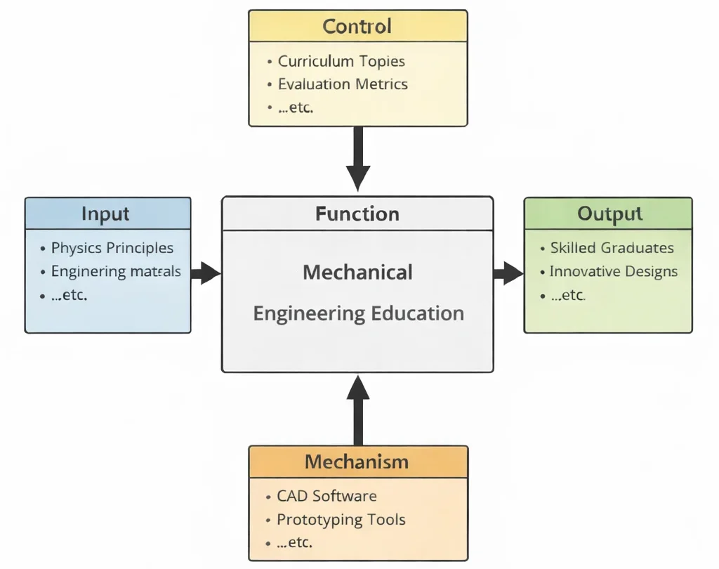
Inputs (Left): Fundamental physical principles, raw empirical load data, multiaxial stress states, operational duty cycles, and real-world system boundary conditions.
Controls (Top): Washington Accord/EUR-ACE accreditation frameworks, ISO/ASME/ASTM engineering standards, safety factors (SF), geometric dimensioning & tolerancing (GD&T), and sustainability mandates.
Mechanisms (Bottom): High-performance computing nodes, finite element solvers (FEA/CFD), metrology laboratories, additive/subtractive tooling, and cyber-physical telemetry testbeds.
Outputs (Right): Validated mechanical architectures, certified safety-critical components, closed-loop control algorithms, verified thermal-fluid balances, and practice-ready engineering leadership.

Mechanical Engineering Curricular Specializations

Select any foundational pillar below to access dedicated derivations, computational tools, and deep-dive practice modules within the Prep4Uni Mechanical Engineering cluster:

Current Topic

Mechanical Engineering (Curricular Hub)

Central foundation integrating energy conservation, machine kinematic synthesis, material limits, and dynamic control.

Mobility Systems

Automotive Engineering

Applies core mechanical thermodynamics, chassis kinematics, and structural impact mechanics to vehicle design.

Medical Mechanics

Biomechanical Engineering

Translates mechanical stress, continuum mechanics, and kinematic linkages into prosthetic and human biological systems.

Feedback & Stability

Control Systems in Mechanical Engineering

Closes the loop on mechanical systems using sensors, actuators, and dynamic state-space controllers.

Fluid Dynamics

Fluid Mechanics and Hydraulics

Governs internal and external momentum transport, piping hydraulic losses, and Navier-Stokes boundary flows.

Industrial Fabrication

Manufacturing and Production Engineering

Transforms theoretical CAD models into real products via machining, forming, additive processes, and metrology.

Digital Design

Mechanical Design and CAD

Executes geometric dimensioning, parametric feature modeling, and structural assembly synthesis in digital space.

Advanced Materials

Nanotechnology and Advanced Materials

Engineers micro- and nano-scale material grain boundaries, nanocomposites, and thermal barrier enhancements.

Robotic Systems

Robotics and Automation in Mechanical Engineering

Combines mechanical linkage dynamics with multi-axis trajectory planning and industrial automation.

Structural Mechanics

Solid Mechanics: Stress, Strain & Structural Analysis

Analyzes elastic and plastic stress distributions, Mohr’s circle transformations, and structural failure criteria.

Thermal Science

Thermodynamics and Heat Transfer

Quantifies energy conversion efficiency, second-law exergy destruction, and multi-mode heat transport.

Wave Dynamics

Vibrations and Acoustics

Evaluates oscillatory structural responses, resonance limits, modal shapes, and acoustic noise radiation.

Advanced engineering laboratory showing FEA dashboards, automated robotic arms, and CAD systems.

Figure 2.0: Contemporary mechanical engineering workspace: integration of numerical simulation, robotics, and cyber-physical prototyping.

Deep Technical Foundations: Governing Analytical Formulations

Mechanical engineering solves physical challenges across macroscopic and microscopic scales by translating boundary-value problems into mathematical formulations. Mastery of the discipline requires rigorous fluency across solid, fluid, and thermodynamic governing frameworks.

1. Continuum Solid Mechanics & Euler-Bernoulli Beam Deflection

For an isotropic, linear-elastic structural member where transverse shear strains are negligible (L/h > 10), the flexural deflection v(x) is governed by the fourth-order ordinary differential equation:

$$EI \frac{d^4 v(x)}{dx^4} = q(x)$$

where E represents Young's Modulus of Elasticity in N/m², I is the second moment of area in m⁴, and q(x) is the distributed transverse load in N/m. For a simply supported prismatic beam of length L subjected to a central point load P at x = L/2, integrating under kinematic boundary conditions (v(0) = 0, v(L) = 0, M(0) = 0, M(L) = 0) yields the elastic displacement profile for 0 ≤ x ≤ L/2:

$$v(x) = \frac{P x}{48 E I} \left(3L^2 - 4x^2\right)$$

Evaluating this at mid-span (x = L/2) gives the peak structural deflection (δ_max):

$$\delta_{\max} = \frac{P L^3}{48 E I}$$

Simultaneously, the internal bending moment is M(x) = (P · x)/2 for 0 ≤ x ≤ L/2, reaching a peak at mid-span of M_max = (P · L)/4. The extreme outer-fiber flexural stress is calculated via the elastic section modulus Z = I/c:

$$\sigma_{\max} = \frac{M_{\max} c}{I} = \frac{P L c}{4 I}$$

2. Viscous Fluid Dynamics: Incompressible Navier-Stokes Equations

The conservation of linear momentum for a Newtonian, incompressible fluid of constant dynamic viscosity μ and density ρ is expressed by the vector Navier-Stokes formulation:

$$\rho \left( \frac{\partial \mathbf{u}}{\partial t} + (\mathbf{u} \cdot \nabla) \mathbf{u} \right) = -\nabla p + \mu \nabla^2 \mathbf{u} + \rho \mathbf{g}$$

paired with the continuity requirement ∇ · u = 0. In internal pressurized conduits, the frictional head loss h_f over span L and diameter D is quantified by the Darcy-Weisbach formulation:

$$h_f = f \cdot \frac{L}{D} \cdot \frac{v^2}{2g}$$

where the Darcy friction factor f is a function of the Reynolds number Re = (ρ · v · D) / μ and relative wall roughness ε/D, transitioning from laminar behavior (f = 64/Re when Re < 2300) to fully turbulent flow governed by the implicit Colebrook-White relationship:

$$\frac{1}{\sqrt{f}} = -2 \log_{10} \left( \frac{\varepsilon / D}{3.7} + \frac{2.51}{\text{Re} \sqrt{f}} \right)$$

3. Thermal Energy Conservation & Thermodynamic Cycles

The differential energy balance equation for multi-dimensional heat conduction with internal thermal generation rate per unit volume q̇_g is formulated by Fourier's law combined with internal energy storage:

$$\rho c_p \frac{\partial T}{\partial t} = \nabla \cdot (k \nabla T) + \dot{q}_g$$

For cyclic heat engines operating between an isothermal high-temperature source (T_H) and sink (T_C), the Second Law of Thermodynamics enforces the Carnot upper limit on thermal conversion efficiency (η_th):

$$\eta_{\text{th}} = \frac{W_{\text{net}}}{Q_{\text{in}}} \le \eta_{\text{Carnot}} = 1 - \frac{T_C}{T_H}$$

Contemporary Computational Paradigms in Modern Practice

Modern engineering design has moved beyond purely empirical testing or uncoupled numerical solvers. Contemporary mechanical workflows operate within coupled digital frameworks that merge physical conservation laws with high-speed digital architectures:

Physics-Informed Neural Networks (PINNs)

By embedding partial differential equations (such as the Navier-Stokes or Biharmonic elasticity equations) directly into deep learning loss functions (L_total = L_data + λL_PDE), PINNs solve complex inverse problems and characterize non-destructive material degradation with sparse experimental sensor data.

Fourier Neural Operators (FNOs)

Parametric PDE solvers operating in Fourier space map entire continuous input function fields to full solution spaces. FNOs execute turbulent flow CFD evaluations and nonlinear thermal evaluations up to three orders of magnitude faster than traditional fine-mesh numerical solvers, making them ideal for rapid iterative generative design.

Discrete-Event Digital Twins & Telemetry

Industrial mechanical systems combine physical components with real-time operational models. Onboard IoT vibration, strain, and temperature telemetry continually update reduced-order models (ROMs) via Extended Kalman Filtering to execute predictive failure modeling and dynamic fatigue lifecycle tracking.

Systems Engineering Trade-off Matrix

Every mechanical engineering decision involves managing conflicting requirements. The matrix below outlines fundamental design strategies, their benefits, operational risks, and industry-standard mitigations:

Design / System Strategy	Primary Engineering Advantage	Bottlenecks & Failure Modes	Mitigation & Control Strategy
High-Yield Thin-Walled Structures	Substantial mass reduction; optimizes specific strength (σ_y / ρ); minimizes energy consumption in automotive/aerospace systems.	Heightened vulnerability to elastic buckling, localized crippling, reduced second moment of area (I), and accelerated high-cycle vibration fatigue.	Incorporate internal stiffening ribs; use topology optimization; perform nonlinear eigenvalue buckling analysis with safety factor SF ≥ 2.0.
Monolithic Additive Manufacturing (AM)	Eliminates fasteners, seals, and braze joints; enables complex internal conformal cooling channels and consolidated multi-part assemblies.	Anisotropic grain structures along build orientations; residual tensile stresses; micro-voids; severe surface roughness acting as fatigue stress risers.	Execute Hot Isostatic Pressing (HIP) heat treatments; apply abrasive flow surface polishing; orient critical principal stress vectors along build planes.
High-Compression Thermodynamic Cycles	Maximizes thermal conversion efficiency (η_th) via elevated expansion ratios; compact power-density footprints.	Severe thermal-mechanical creep; rapid thermal barrier coating (TBC) spallation; elevated NO_x emissions due to high peak temperatures.	Deploy single-crystal nickel-based superalloys with internal serpentine cooling paths; use ceramic matrix composites (CMCs) and advanced closed-loop lean burn controls.
Active Cyber-Physical Feedback Control	Compensates for structural deflections and dynamic disturbances in real time; enables flexible, ultra-lightweight structural configurations.	Actuator saturation; sensor noise injection; time-delay phase lag driving the closed-loop system into catastrophic resonance or instability.	Design robust H_∞ controllers with conservative gain/phase margins; implement physical mechanical fail-safes (end-stops, dampers) and dual-redundant bus architectures.

Cross-Sector Industrial Case Studies

Aerospace Propulsion

Turbofan engine high-pressure turbine blades operate in gas temperatures exceeding 1700 K—well above the melting point of bare nickel alloys. Mechanical engineers solve this by designing intricate internal film-cooling channels and applying yttria-stabilized zirconia (YSZ) thermal barrier coatings.

Electric Mobility

Battery enclosures in electric vehicles must serve as structural shear panels during high-g collisions while isolating hundreds of lithium-ion cells from thermal runaway. This requires balanced crashworthiness design, die-cast aluminum alloys, and integrated liquid cold-plate heat exchangers.

Precision Semiconductor Tools

Photolithography wafer steppers demand sub-nanometer positioning at dynamic accelerations exceeding 10g. Mechanical engineers use magnetically levitated planar stages, Zerodur low-expansion glass ceramics, and active vibration isolation tables.

Offshore Wind Turbines

Turbine blades over 100 meters in length encounter cyclic aeroelastic flutter, gravitational fatigue, and harsh salt-spray corrosion. Engineers use carbon-glass hybrid composite laminates, passive bend-twist coupling, and tuned mass dampers inside the nacelle.

Interactive Simulation: Euler-Bernoulli Elastic Beam Bending

Evaluate real-time structural deflection and internal moment distributions under concentrated transverse loading. This simulation models a simply supported beam with user-selected structural parameters, applying Euler-Bernoulli beam theory via our verified zero-crash canvas architecture.

Euler-Bernoulli Elastic Flexure Engine

STATUS: ACTIVE SOLVER

Applied Load P: 5000 N

Span Length L: 3.0 m

Elastic Modulus E: 200 GPa

Moment of Inertia I: 10.0 × 10⁻⁶ m⁴

Max Deflection (δ_max)

0.70 mm

Peak Moment (M_max)

3,750 N·m

Flexural Rigidity (EI)

2.00 MN·m²

Elastic Deflection Profile v(x) Bending Moment Envelope M(x)

Frequently Asked Questions: Curricular & Professional Standards

1. What distinguishes the Washington Accord engineering standard from basic technology diplomas?

The Washington Accord recognizes substantial equivalence in engineering degree programs based on complex problem solving and complex engineering activities. Unlike prescriptive, technician-level technology curricula that focus on standard operating procedures, an Accord-accredited mechanical curriculum demands mathematical modeling from first principles (such as continuum mechanics, vector differential calculus, and partial differential equations), analytical derivation under conflicting operational constraints, and defensible engineering judgment.

2. How do modern mechanical engineers balance analytical derivations with commercial FEA/CFD packages?

Commercial simulation software (ANSYS, Abaqus, COMSOL, Star-CCM+) uses numerical discretization to approximate solutions for complex geometries. However, relying on these tools without analytical grounding often leads to unverified, error-prone results. Professional engineers use closed-form equations (such as Euler-Bernoulli beam theory, thick-walled cylinder equations, or 1D flat-plate thermal resistances) to complete order-of-magnitude hand calculations before running numerical models. These manual checks establish mesh convergence criteria, flag invalid boundary conditions, and verify that solutions are physically reasonable.

3. Why is Euler-Bernoulli beam theory valid only under specific slenderness ratios?

Euler-Bernoulli theory rests on the kinematic assumption that cross-sections remain plane and perpendicular to the deformed neutral axis (γ_xz = 0). This holds true for slender members where the span-to-depth ratio exceeds approximately 10 (L/h > 10). For short, deep beams (L/h < 10), transverse shear deformation becomes significant, requiring Timoshenko beam theory to avoid underestimating true physical deflections.

4. What role does Geometric Dimensioning & Tolerancing (GD&T) play in machine design?

Governed by standards like ASME Y14.5 and ISO 1101, GD&T defines allowable geometry variations through precise datum reference frames and functional tolerance zones (e.g., true position, flatness, runout, perpendicularity). Unlike simple linear plus/minus tolerances, GD&T communicates design intent based on part function, ensures interchangeability during high-volume assembly, and reduces manufacturing costs by expanding permissible variations without compromising assembly fit.

5. How does the von Mises yield criterion differ from the Maximum Shear Stress (Tresca) criterion?

Both criteria evaluate ductile yielding under multiaxial stress states. The Tresca criterion assumes failure occurs when maximum absolute shear stress matches the shear stress at yield in simple tension (τ_max ≥ σ_y / 2), which produces a conservative hexagonal yield locus. The von Mises criterion evaluates distortion energy density: $$\sigma_v = \sqrt{\frac{1}{2} \left[ (\sigma_1 - \sigma_2)^2 + (\sigma_2 - \sigma_3)^2 + (\sigma_3 - \sigma_1)^2 \right]} \ge \sigma_y$$ This yields an elliptical locus that aligns more closely with experimental data for ductile metals, allowing for more mass-efficient designs while maintaining structural safety.

6. How does the First Law differ from the Second Law of Thermodynamics in energy systems design?

The First Law governs the quantity of energy, establishing that energy is conserved across thermal, work, and mass-flow boundaries (ΔE = Q − W). The Second Law governs the quality and direction of energy flow, establishing that isolated systems experience non-negative entropy generation (S_gen ≥ 0). While the First Law allows for 100% heat-to-work conversion, the Second Law establishes the Carnot efficiency limit, proving that heat cannot be converted into net work in a cyclic process without rejecting waste heat to a lower-temperature sink.

7. What is the difference between finite element analysis (FEA) and finite volume method (FVM)?

FEA divides structural domains into finite elements, using variational formulations (such as the principle of virtual work and Galerkin weighted residuals) to solve displacement fields and stress tensors. FVM divides fluid regions into small control volumes, integrating conservative governing equations directly across every face: $$\int_S (\mathbf{F} \cdot \mathbf{n}) \, dA = \int_V S_V \, dV$$ Because FVM strictly enforces mass, momentum, and energy conservation across every discrete cell, it is the primary method used in computational fluid dynamics.

8. How do digital twins transition from reactive monitoring to predictive lifecycle maintenance?

A basic monitoring platform simply displays live telemetry like vibration or temperature. A true digital twin couples live sensor feeds with physics-based models (such as Paris-Erdogan crack-growth formulations and transient thermal models). By applying Bayesian estimation or Extended Kalman Filtering, the twin calculates real-time damage accumulation and remaining useful life (RUL), shifting maintenance schedules from fixed calendar intervals to actual component health needs.

Student Practice & Accreditation Assessment Modules

Section 1: Conceptual Knowledge Self-Assessment

Q1: Explain why a circular cross-section is mathematically superior for pure torsional transmission compared to a thin rectangular section.

A circular shaft maintains axisymmetric shear strain distributions under pure torsion; planar cross-sections rotate as rigid bodies without experiencing out-of-plane warping. In non-circular cross-sections (such as thin rectangles), torsional shear stresses cause significant warping displacements out of the plane. Restrained warping generates severe corner stress concentrations, and because shear stresses drop to zero at the corners and peak along the flat boundaries, non-circular geometries require much more material to achieve the same torsional stiffness and load capacity.

Q2: Formulate the physical significance of the Reynolds number in dynamic fluid regimes.

The Reynolds number represents the dimensionless ratio of convective inertial forces to viscous resistive shear forces: $$\text{Re} = \frac{\rho v D}{\mu} = \frac{\text{Inertial Forces}}{\text{Viscous Forces}}$$ When Re ≪ 2300, viscous damping dominates, stabilizing perturbations into smooth, laminar streamlines. When Re ≫ 4000, inertial forces overcome viscous damping, allowing small disturbances to amplify into turbulent, swirling eddies with broad energy-cascade spectra.

Q3: Why does adding cooling fins beyond a critical thickness or length reduce, rather than increase, total heat rejection?

While adding fin surface area (A_s) increases convective dissipation (q = h · A_s · ΔT), the heat must first travel through the fin via conduction. Long, thin fins introduce substantial internal conductive thermal resistance (R_cond = L / (k · A_c)). As conduction resistance grows, the fin surface temperature drops toward the ambient fluid temperature, lowering the effective thermal driving potential (ΔT). Beyond a design threshold, the added conductive resistance and boundary layer interference outweigh the surface area gains, lowering the fin efficiency (η_f) and reducing overall system heat transfer.

Q4: How do the Soderberg, Goodman, and Gerber fatigue criteria differ when designing against fluctuating cyclic loads?

All three criteria plot fluctuating mean stress (σ_m) on the horizontal axis against alternating stress amplitude (σ_a) on the vertical axis:

Soderberg: Connects endurance limit S_e to yield strength S_y: $$\frac{\sigma_a}{S_e} + \frac{\sigma_m}{S_y} = 1$$ It provides the most conservative safety margins, guarding against both fatigue and static yielding.
Modified Goodman: Connects endurance limit S_e to ultimate tensile strength S_ut: $$\frac{\sigma_a}{S_e} + \frac{\sigma_m}{S_{ut}} = 1$$ This is the standard industrial baseline for ductile metals under cyclical tensile stress.
Gerber: Uses a parabolic relationship connecting S_e to S_ut: $$\frac{\sigma_a}{S_e} + \left(\frac{\sigma_m}{S_{ut}}\right)^2 = 1$$ It models real experimental fatigue failure data closely, but provides smaller safety margins when positive mean stresses are present.

Q5: Why is the thermal boundary layer thicker than the velocity boundary layer when the Prandtl number is less than unity?

The dimensionless Prandtl number compares momentum diffusivity to thermal diffusivity: $$\text{Pr} = \frac{\nu}{\alpha} = \frac{\mu / \rho}{k / (\rho c_p)}$$ For liquid metals (such as sodium-potassium mixtures where Pr ≪ 1), molecular thermal conductivity is exceptionally high relative to viscosity. Heat conducts outward through the fluid much faster than viscous shear forces propagate momentum, resulting in a thermal boundary layer thickness (δ_t) that is significantly larger than the velocity boundary layer thickness (δ).

Q6: Differentiate between ductile and brittle fracture modes under high-strain impact loading.

Ductile fractures involve extensive plastic deformation, microvoid nucleation, growth, and coalescence. This creates rough, fibrous fracture surfaces and distinct macroscopic necking, which absorbs substantial strain energy prior to final separation. Brittle fractures occur with minimal plastic deformation via rapid transgranular cleavage or intergranular cracking along crystallographic planes. Brittle failures produce flat, reflective fracture surfaces that propagate at speeds near the speed of sound, often triggered when operational temperatures drop below the material's ductile-to-brittle transition temperature (DBTT).

Q7: Why do underdamped mechanical vibrating systems experience maximum resonant displacement below the undamped natural frequency?

For a standard single-degree-of-freedom mass-spring-damper system, the undamped natural frequency is ω_n = √(k/m). In the presence of viscous damping (damping ratio 0 < ζ < 1/√2), the peak dynamic magnification factor occurs at the resonant forcing frequency: $$\omega_r = \omega_n \sqrt{1 - 2\zeta^2}$$ Energy dissipation from the viscous damper continuously shifts the phase angle between excitation and displacement, so the maximum steady-state response amplitude occurs slightly below ω_n.

Q8: What physical mechanisms cause cavitation in centrifugal pumps, and how does Net Positive Suction Head (NPSH) prevent it?

Cavitation occurs when localized static fluid pressure drops below the vapor pressure (p_v) at the operating temperature, typically near the high-velocity suction eye of an impeller. This low pressure vaporizes the liquid into vapor bubbles. As these bubbles enter higher-pressure impeller regions, they collapse violently within microseconds, generating micro-jets with localized pressures up to several gigapascals that pit and erode the metal surfaces. To prevent this, systems must maintain a Net Positive Suction Head Available (NPSH_A) that exceeds the manufacturer's required suction head (NPSH_R) by a defined margin: $$\text{NPSH}_A = \frac{p_{\text{inlet}} - p_v}{\rho g} + \frac{v_{\text{inlet}}^2}{2g} > \text{NPSH}_R$$

Section 2: Analytical & Scenario-Based Case Studies

Case Study 2.1: Fatigue-Induced Turbine Shaft Fracture in Combined Bending and Torsion POWER GENERATION

Scenario: A 120-mm-diameter solid AISI 4340 alloy steel driveshaft on an auxiliary steam turbine failed catastrophically after 14 months of operation[cite: 1]. Fracture analysis revealed beach marks originating at a 1.5-mm shoulder radius fillet, indicating progressive fatigue that transitioned to fast brittle fracture across 65% of the cross-section[cite: 1].

Engineering Evaluation:
1. Stress Concentration: The sharp transition fillet generated a localized geometric stress concentration factor (K_t ≈ 2.4), which raised localized cyclical stresses well above the alloy's endurance limit (S_e)[cite: 1].
2. Multiaxial Loading: The shaft experienced steady torsional shear from electrical generation combined with fully reversed cyclic bending caused by slight bearing misalignment[cite: 1]. This produced an alternating multiaxial stress state[cite: 1]: $$\sigma_{a,\text{eq}} = \sqrt{\sigma_a^2 + 3\tau_a^2}$$
Corrective Engineering Action: Redesign the shoulder fillet radius from 1.5 mm to 6.0 mm (reducing K_t to 1.35), introduce deep-roll burnishing to generate protective compressive residual surface stresses, and install laser-aligned hydrodynamic bearings monitored by online spectral vibration sensors[cite: 1].

Case Study 2.2: Thermal Runaway Propagation in Structural EV Battery Enclosures AUTOMOTIVE MOBILITY

Scenario: During ground-strike testing of an electric vehicle pack, road debris penetrated an underbody aluminum skid plate, puncturing an internal 2170 cylindrical cell[cite: 2]. Within 45 seconds, the cell triggered an exothermic cascade that compromised adjacent cells through conductive thermal runaway[cite: 2].

Engineering Evaluation:
1. Structural Impact Resistance: The original single-layer 6000-series aluminum base lacked adequate dynamic shear resistance under high-velocity localized impacts[cite: 2].
2. Thermal Isolation: The cell-to-cell structural bonding adhesive had high thermal conductivity, which allowed rapid propagation of a 900°C thermal wave to neighboring cells[cite: 2].
Corrective Engineering Action: Upgrade to a dual-phase ultra-high-strength steel (UHSS) sandwich baseplate with an energy-absorbing honeycomb core[cite: 2]. Isolate individual cells with aerogel insulation pads (k ≈ 0.018 W/(m·K)), and route rapid-discharge directional pyrotechnic venting channels through the pack roof[cite: 2].

Case Study 2.3: Water Hammer Rupture in a High-Head Hydroelectric Penstock HYDRAULIC INFRASTRUCTURE

Scenario: Following a grid-trip event, an emergency shut-off butterfly valve on an 800-meter welded steel penstock closed in 1.2 seconds[cite: 2]. The sudden deceleration caused a hydraulic shock wave that ruptured an upstream welded expansion joint, flooding the turbine hall[cite: 2].

Engineering Evaluation:
1. Wave Travel Mechanics: The acoustic pressure wave speed through the water-filled elastic steel pipe was[cite: 2]: $$a = \sqrt{\frac{K / \rho}{1 + (K/E)(D/t)}} \approx 1050 \text{ m/s}$$ The critical pipeline reflection period was 2L/a = 2(800)/1050 ≈ 1.52 s[cite: 2]. Because the valve closed in t_c = 1.2 s < 2L/a, the event behaved as an abrupt closure, generating a Joukowsky pressure surge[cite: 2]: $$\Delta p = \rho \cdot a \cdot \Delta v$$ With an initial flow velocity change of Δv = 4.2 m/s, the surge pressure was[cite: 2]: $$\Delta p = 1000 \cdot 1050 \cdot 4.2 = 4.41 \times 10^6 \text{ Pa} = 4.41 \text{ MPa} \quad (\approx 450 \text{ m of added head})$$ This transient load exceeded the yield strength of the aged welded joint[cite: 2].
Corrective Engineering Action: Reprogram the valve actuator with a two-stage closure profile (80% closure over 12 seconds, followed by slow final seating over 8 seconds), and install a surge tank near the turbine inlet to absorb fluid momentum[cite: 2].

Case Study 2.4: High-Cycle Aeroelastic Flutter in Transonic Compressor Blisk Assemblies AEROSPACE PROPULSION

Scenario: During high-altitude engine certification flights, titanium integrally bladed rotors (blisks) on a low-pressure compressor experienced blade-tip micro-cracking within 85 flight hours.

Engineering Evaluation:
Unlike traditional slotted blade roots that dissipate vibration through frictional sliding, monolithic blisks have near-zero mechanical damping. At transonic speeds, periodic shock-wave oscillations on the suction surfaces coupled with the first torsional structural mode of the blades. This aeroelastic flutter drove rapid cyclic strain accumulation and high-cycle fatigue failure.
Corrective Engineering Action: Modify blade geometry to introduce intentional aerodynamic sweep (disrupting coherent spanwise shock oscillations), and apply ring dampers inside the blisk rim to reintroduce friction-based damping.

Case Study 2.5: Thermal Fatigue Cracking in Regenerative Rocket Nozzle Channels SPACE PROPULSION

Scenario: A reusable liquid oxygen/methane rocket engine prototype developed microscopic coolant-channel cracks after four static hot-fire cycles, allowing fuel to leak into the expansion plume.

Engineering Evaluation:
The copper-alloy (GRCop-84) inner liner undergoes extreme thermal gradients across its 0.8-mm hot-gas wall (outer face ∼ 850 K, coolant-wetted face ∼ 180 K). The constrained thermal expansion generates cyclic compressive plastic strain during firing, followed by tensile residual stresses upon shutdown. This rapid thermal cycle caused low-cycle thermal fatigue cracking.
Corrective Engineering Action: Electroplate a 50-μm ductile nickel barrier layer within the milled cooling channels, optimize channel aspect ratios to reduce peak wall temperatures, and introduce a fuel-film cooling layer along the nozzle interior boundary layer.

Case Study 2.6: Harmonic Resonance Breakdown in an Industrial Chiller Variable-Speed Compressor HVAC & BUILDING INFRASTRUCTURE

Scenario: A variable-speed centrifugal water chiller installed on a hospital rooftop experienced severe vibration and pipe flange cracking whenever the motor modulated to 48.5 Hz (2910 RPM).

Engineering Evaluation:
Modal tap testing identified a natural frequency of the chiller's structural base frame and discharge piping at 48.8 Hz, with a low damping ratio (ζ ≈ 0.012). When the motor operated near 48.5 Hz, rotational unbalance excited the frame into resonance, driving vibration amplitudes above 18 mm/s RMS (exceeding ISO 10816 limits).
Corrective Engineering Action: Stiffen the structural steel base with diagonal gusset plates (raising the natural frequency to 61 Hz, well outside the operating range), install elastomeric vibration isolation pads with ζ ≥ 0.08, and program a frequency exclusion band (46–51 Hz) into the variable frequency drive (VFD).

Case Study 2.7: Stress-Corrosion Cracking in an Offshore Subsea Wellhead Connector ENERGY & OFFSHORE EXTRACTION

Scenario: A subsea locking mandrel forged from high-strength martensitic stainless steel failed after three years of deepwater service, despite operating well within its static design yield limits.

Engineering Evaluation:
Failure occurred through Chloride-Induced Stress-Corrosion Cracking (CISCC). The mandrel operated under sustained tensile preload stress in a high-chloride marine environment, while cathodic protection produced hydrogen embrittlement at localized pit sites. Crack growth followed stress-corrosion mechanisms governed by: $$K_I \ge K_{\text{ISCC}}$$
Corrective Engineering Action: Replace the material with cold-worked Inconel 718 (a nickel-chromium superalloy with superior CISCC immunity), lower the bolt torque spec to keep sustained tensile stresses below 40% of yield, and apply thermally sprayed aluminum coatings to improve galvanic protection.

Section 3: Step-by-Step Quantitative Worked Examples

Worked Example 3.1: Deflection and Peak Flexural Stress in an Overhead Crane Girder SOLID MECHANICS

Problem Statement: A simply supported structural steel wide-flange beam spans L = 8.0 m and supports a central hoist load of P = 45 kN. The cross-section has a second moment of area I = 1.25 × 10⁻⁴ m⁴, a total depth 2c = 0.40 m (c = 0.20 m), and Young's Modulus E = 200 × 10⁹ N/m². Calculate:
(a) The maximum mid-span deflection (δ_max) in millimeters.
(b) The peak flexural bending stress (σ_max) at the outer fibers in MPa.
(c) The structural safety factor (SF) if the steel yield strength is σ_y = 250 MPa.

Step 1: Compute Maximum Deflection (δ_max) $$\delta_{\max} = \frac{P L^3}{48 E I} = \frac{(45{,}000 \text{ N}) \cdot (8.0 \text{ m})^3}{48 \cdot (200 \times 10^9 \text{ N/m}^2) \cdot (1.25 \times 10^{-4} \text{ m}^4)}$$ $$\delta_{\max} = \frac{45{,}000 \cdot 512}{48 \cdot 200 \times 10^9 \cdot 1.25 \times 10^{-4}} = \frac{23{,}040{,}000}{1{,}200{,}000{,}000} = 0.0192 \text{ m} = 19.20 \text{ mm}$$

Step 2: Compute Maximum Bending Moment (M_max) $$M_{\max} = \frac{P L}{4} = \frac{(45{,}000 \text{ N}) \cdot (8.0 \text{ m})}{4} = 90{,}000 \text{ N}\cdot\text{m}$$

Step 3: Compute Peak Flexural Stress (σ_max) $$\sigma_{\max} = \frac{M_{\max} c}{I} = \frac{(90{,}000 \text{ N}\cdot\text{m}) \cdot (0.20 \text{ m})}{1.25 \times 10^{-4} \text{ m}^4} = \frac{18{,}000}{1.25 \times 10^{-4}} = 144 \times 10^6 \text{ Pa} = 144.00 \text{ MPa}$$

Step 4: Compute Structural Safety Factor (SF) $$SF = \frac{\sigma_y}{\sigma_{\max}} = \frac{250 \text{ MPa}}{144 \text{ MPa}} \approx 1.74$$

Engineering Interpretation: The calculated deflection ratio (δ / L = 19.2 / 8000 ≈ 1 / 416) satisfies the standard overhead crane deflection limit (≤ L/400), preventing hoist trolley jamming. The safety factor of 1.74 against yielding confirms the design is safe for static loads, though cyclic hoist operations require a separate fatigue life assessment.

Worked Example 3.2: Torsional Shear Stress and Angular Twist in a Propulsion Driveshaft MACHINE DESIGN

Problem Statement: A marine diesel engine delivers P_mech = 450 kW at an operational speed of N = 1800 RPM to a solid steel driveshaft of length L = 3.5 m and radius r = 0.04 m (diameter D = 0.08 m). The material shear modulus is G = 78 GPa. Calculate:
(a) The operational torque (T) transmitted by the shaft.
(b) The peak surface shear stress (τ_max) in MPa.
(c) The total torsional elastic twist (θ) across the shaft in degrees.

Step 1: Compute Applied Torque (T) $$\omega = \frac{2 \pi N}{60} = \frac{2 \pi \cdot 1800}{60} = 60 \pi \approx 188.496 \text{ rad/s}$$ $$T = \frac{P_{\text{mech}}}{\omega} = \frac{450{,}000 \text{ W}}{188.496 \text{ rad/s}} \approx 2387.32 \text{ N}\cdot\text{m}$$

Step 2: Compute Polar Moment of Inertia (J) $$J = \frac{\pi}{2} r^4 = \frac{\pi}{2} (0.04 \text{ m})^4 = \frac{\pi}{2} (2.56 \times 10^{-6}) \approx 4.0212 \times 10^{-6} \text{ m}^4$$

Step 3: Compute Maximum Surface Shear Stress (τ_max) $$\tau_{\max} = \frac{T r}{J} = \frac{(2387.32 \text{ N}\cdot\text{m}) \cdot (0.04 \text{ m})}{4.0212 \times 10^{-6} \text{ m}^4} = \frac{95.4928}{4.0212 \times 10^{-6}} \approx 23{,}747{,}100 \text{ Pa} \approx 23.75 \text{ MPa}$$

Step 4: Compute Torsional Angular Twist (θ) $$\theta_{\text{rad}} = \frac{T L}{J G} = \frac{(2387.32 \text{ N}\cdot\text{m}) \cdot (3.5 \text{ m})}{(4.0212 \times 10^{-6} \text{ m}^4) \cdot (78 \times 10^9 \text{ N/m}^2)} = \frac{8355.62}{313{,}653.6} \approx 0.02664 \text{ rad}$$ $$\theta_{\text{deg}} = 0.02664 \text{ rad} \cdot \left(\frac{180^\circ}{\pi}\right) \approx 1.526^\circ$$

Engineering Interpretation: The maximum shear stress of 23.75 MPa is well below the allowable shear limit for typical shaft steels (τ_allow ≈ 50–70 MPa). The total twist of 1.53° over 3.5 meters (0.44°/m) falls within standard limits (< 0.5°/m), ensuring the shaft will not cause gear misalignment or driveline vibration.

Worked Example 3.3: Darcy-Weisbach Friction Head Loss in an Industrial Cooling Loop FLUID DYNAMICS

Problem Statement: Water at 20°C (density ρ = 998 kg/m³, dynamic viscosity μ = 1.002 × 10⁻³ Pa·s) flows through a horizontal commercial steel pipe (diameter D = 0.15 m, absolute roughness ε = 0.045 mm) of length L = 120 m at a volumetric flow rate Q = 0.055 m³/s[cite: 3]. Given acceleration due to gravity g = 9.81 m/s²[cite: 3]:
(a) Determine the mean flow velocity (v) and Reynolds number (Re)[cite: 3].
(b) Determine the Darcy friction factor (f) using the Swamee-Jain explicit approximation[cite: 3].
(c) Calculate total frictional head loss (h_f) and the required pumping power (P_pump) assuming 100% pump efficiency[cite: 3].

Step 1: Compute Flow Velocity and Reynolds Number $$A = \frac{\pi D^2}{4} = \frac{\pi (0.15)^2}{4} \approx 0.017671 \text{ m}^2$$ $$v = \frac{Q}{A} = \frac{0.055}{0.017671} \approx 3.112 \text{ m/s}$$ $$\text{Re} = \frac{\rho v D}{\mu} = \frac{(998) \cdot (3.112) \cdot (0.15)}{1.002 \times 10^{-3}} = \frac{465.866}{1.002 \times 10^{-3}} \approx 464{,}936 \quad (\text{Fully Turbulent})$$

Step 2: Compute Darcy Friction Factor (f) $$\frac{\varepsilon}{D} = \frac{0.045 \times 10^{-3} \text{ m}}{0.15 \text{ m}} = 0.00030$$ $$f = \frac{0.25}{\left[ \log_{10} \left( \frac{\varepsilon/D}{3.7} + \frac{5.74}{\text{Re}^{0.9}} \right) \right]^2} = \frac{0.25}{\left[ \log_{10} \left( \frac{0.00030}{3.7} + \frac{5.74}{(464936)^{0.9}} \right) \right]^2}$$ $$\frac{0.00030}{3.7} \approx 8.108 \times 10^{-5}, \quad \frac{5.74}{122{,}857} \approx 4.672 \times 10^{-5}$$ $$\text{Sum} \approx 1.278 \times 10^{-4} \Longrightarrow \log_{10}(1.278 \times 10^{-4}) \approx -3.8935$$ $$f = \frac{0.25}{(-3.8935)^2} = \frac{0.25}{15.159} \approx 0.01649$$

Step 3: Compute Head Loss (h_f) and Pressure Drop (Δp) $$h_f = f \cdot \frac{L}{D} \cdot \frac{v^2}{2g} = (0.01649) \cdot \left(\frac{120}{0.15}\right) \cdot \left(\frac{(3.112)^2}{2 \cdot 9.81}\right) = (0.01649) \cdot (800) \cdot \left(\frac{9.6845}{19.62}\right) \approx 6.509 \text{ m}$$ $$\Delta p = \rho g h_f = (998) \cdot (9.81) \cdot (6.509) \approx 63{,}725 \text{ Pa} = 63.73 \text{ kPa}$$

Step 4: Compute Theoretical Pumping Power (P_pump) $$P_{\text{pump}} = \Delta p \cdot Q = (63{,}725 \text{ N/m}^2) \cdot (0.055 \text{ m}^3/\text{s}) \approx 3504.9 \text{ W} \approx 3.50 \text{ kW}$$

Engineering Interpretation: Overcoming pipe friction requires 3.50 kW of fluid power. Assuming a typical industrial pump-motor efficiency of η_combined ≈ 72%, the facility must install an electrical motor rated for at least P_elec = 3.50 / 0.72 ≈ 4.86 kW (specifying a standard 5.5-kW commercial drive).

Worked Example 3.4: Multi-Layer Thermal Conduction and Insulation Sizing THERMODYNAMICS & HEAT TRANSFER

Problem Statement: An industrial furnace wall consists of an inner refractory firebrick layer (L₁ = 0.12 m, k₁ = 1.4 W/(m·K)) and an outer mineral wool insulation layer (k₂ = 0.05 W/(m·K)). The furnace interior surface is maintained at T_hot = 920°C (1193.15 K), and the ambient factory air is at T_∞ = 25°C (298.15 K) with an external natural convection coefficient h_conv = 12 W/(m²·K).
Calculate the minimum mineral wool thickness (L₂) needed to keep the outer casing temperature (T_surface) at or below 55°C (328.15 K) for personnel burn safety.

Step 1: Compute Allowable Surface Heat Flux (q'')

At steady state, the heat flux conducted through the wall equals the heat flux convected from the outer surface to the ambient air:

$$q'' = h_{\text{conv}} (T_{\text{surface}} - T_\infty) = (12 \text{ W/m}^2\cdot\text{K}) \cdot (55^\circ\text{C} - 25^\circ\text{C}) = 12 \cdot 30 = 360 \text{ W/m}^2$$

Step 2: Express Overall Thermal Resistance per Unit Area (R''_total) $$R''_{\text{total}} = \frac{T_{\text{hot}} - T_\infty}{q''} = \frac{920 - 25}{360} = \frac{895}{360} \approx 2.4861 \text{ m}^2\cdot\text{K/W}$$

The total thermal resistance is the sum of the conduction and external convection resistances:

$$R''_{\text{total}} = R''_{\text{firebrick}} + R''_{\text{insulation}} + R''_{\text{convection}} = \frac{L_1}{k_1} + \frac{L_2}{k_2} + \frac{1}{h_{\text{conv}}}$$

Step 3: Solve for Required Insulation Thickness (L₂) $$R''_{\text{firebrick}} = \frac{0.12}{1.4} \approx 0.0857 \text{ m}^2\cdot\text{K/W}$$ $$R''_{\text{convection}} = \frac{1}{12} \approx 0.0833 \text{ m}^2\cdot\text{K/W}$$ $$R''_{\text{insulation}} = R''_{\text{total}} - R''_{\text{firebrick}} - R''_{\text{convection}} = 2.4861 - 0.0857 - 0.0833 = 2.3171 \text{ m}^2\cdot\text{K/W}$$ $$L_2 = R''_{\text{insulation}} \cdot k_2 = (2.3171 \text{ m}^2\cdot\text{K/W}) \cdot (0.05 \text{ W/m}\cdot\text{K}) \approx 0.1159 \text{ m} \approx 115.9 \text{ mm}$$

Engineering Interpretation: To keep the outer surface temperature below 55°C per OSHA safety guidelines, the furnace wall requires a minimum mineral wool insulation thickness of 115.9 mm (specifying standard 120-mm or 125-mm commercial batting). The low thermal conductivity of the mineral wool accounts for 93.2% of the wall's total thermal resistance.

Worked Example 3.5: Carnot and Actual Rankine Thermodynamic Power Cycle Analysis THERMODYNAMICS & HEAT TRANSFER

Problem Statement: A thermal power plant operates between a high-temperature boiler at T_H = 560°C (833.15 K) and a condenser cooled by a river at T_C = 22°C (295.15 K)[cite: 4]. The system consumes fuel input power Q̇_in = 120 MW and produces a net mechanical work output Ẇ_net = 44.5 MW[cite: 4]. Calculate:
(a) The theoretical maximum Carnot thermal efficiency (η_Carnot)[cite: 4].
(b) The actual first-law thermal conversion efficiency (η_actual)[cite: 4].
(c) The Second-Law efficiency (η_II) of the plant[cite: 4].
(d) The rate of waste heat rejection (Q̇_out) discharged into the river[cite: 4].

Step 1: Compute Carnot Efficiency Limit (η_Carnot)[cite: 4] $$\eta_{\text{Carnot}} = 1 - \frac{T_C}{T_H} = 1 - \frac{295.15 \text{ K}}{833.15 \text{ K}} = 1 - 0.35426 = 0.64574 \Longrightarrow 64.57\%$$

Step 2: Compute Actual Thermal Efficiency (η_actual)[cite: 4] $$\eta_{\text{actual}} = \frac{\dot{W}_{\text{net}}}{\dot{Q}_{\text{in}}} = \frac{44.5 \text{ MW}}{120.0 \text{ MW}} \approx 0.37083 \Longrightarrow 37.08\%$$

Step 3: Compute Second-Law Efficiency (η_II)[cite: 4] $$\eta_{\text{II}} = \frac{\eta_{\text{actual}}}{\eta_{\text{Carnot}}} = \frac{0.37083}{0.64574} \approx 0.57427 \Longrightarrow 57.43\%$$

Step 4: Compute Waste Heat Rejection Rate (Q̇_out)[cite: 4] $$\dot{Q}_{\text{out}} = \dot{Q}_{\text{in}} - \dot{W}_{\text{net}} = 120.0 \text{ MW} - 44.5 \text{ MW} = 75.5 \text{ MW}$$

Engineering Interpretation: While the plant achieves an actual thermal efficiency of 37.08%, its Second-Law efficiency of 57.43% reveals that it captures more than half of the thermodynamically available exergy between these two temperature limits[cite: 4]. The remaining losses stem from irreversibilities in the combustion process, piping pressure drops, and turbine blade aerodynamic friction[cite: 4].

Worked Example 3.6: Dynamic Undamped and Damped Resonance Frequencies in Machine Bases VIBRATIONS & DYNAMICS

Problem Statement: An industrial compressor of total mass m = 850 kg is mounted on an elastomeric foundation system with an equivalent stiffness k = 3.2 × 10⁶ N/m and a viscous damping coefficient c = 8.5 × 10³ N·s/m. Calculate:
(a) The undamped natural angular frequency (ω_n) in rad/s and cyclic frequency (f_n) in Hz.
(b) The critical damping coefficient (c_cr) and dimensionless damping ratio (ζ).
(c) The damped natural frequency (f_d) in Hz.
(d) The resonant excitation frequency (f_r) that generates peak displacement amplitude.

Step 1: Compute Undamped Natural Frequency (ω_n, f_n) $$\omega_n = \sqrt{\frac{k}{m}} = \sqrt{\frac{3.2 \times 10^6 \text{ N/m}}{850 \text{ kg}}} = \sqrt{3764.706} \approx 61.357 \text{ rad/s}$$ $$f_n = \frac{\omega_n}{2\pi} = \frac{61.357}{2\pi} \approx 9.765 \text{ Hz}$$

Step 2: Compute Critical Damping and Damping Ratio (ζ) $$c_{\text{cr}} = 2 \sqrt{k \cdot m} = 2 \sqrt{(3.2 \times 10^6) \cdot (850)} = 2 \sqrt{2.72 \times 10^9} = 2 \cdot (52{,}153.6) \approx 104{,}307 \text{ N}\cdot\text{s/m}$$ $$\zeta = \frac{c}{c_{\text{cr}}} = \frac{8500}{104{,}307} \approx 0.08149 \quad (\zeta \lt 1 \Longrightarrow \text{Underdamped System})$$

Step 3: Compute Damped Natural Frequency (f_d) $$\omega_d = \omega_n \sqrt{1 - \zeta^2} = 61.357 \cdot \sqrt{1 - (0.08149)^2} = 61.357 \cdot \sqrt{1 - 0.00664} \approx 61.357 \cdot 0.99667 \approx 61.153 \text{ rad/s}$$ $$f_d = \frac{\omega_d}{2\pi} = \frac{61.153}{2\pi} \approx 9.733 \text{ Hz}$$

Step 4: Compute Resonant Peak Frequency (f_r) $$\omega_r = \omega_n \sqrt{1 - 2\zeta^2} = 61.357 \cdot \sqrt{1 - 2(0.08149)^2} = 61.357 \cdot \sqrt{1 - 0.01328} \approx 61.357 \cdot 0.99334 \approx 60.948 \text{ rad/s}$$ $$f_r = \frac{\omega_r}{2\pi} = \frac{60.948}{2\pi} \approx 9.700 \text{ Hz}$$

Engineering Interpretation: The machine base is lightly underdamped (ζ ≈ 8.15%), placing the resonant frequency (f_r = 9.70 Hz, corresponding to 582 RPM) very close to the undamped natural frequency. To prevent dangerous resonant vibrations during startup and shutdown, the compressor's operating speed must be maintained above √2 f_n ≈ 13.8 Hz (828 RPM), ensuring safe operation in the vibration isolation zone.

Mechanical Engineering