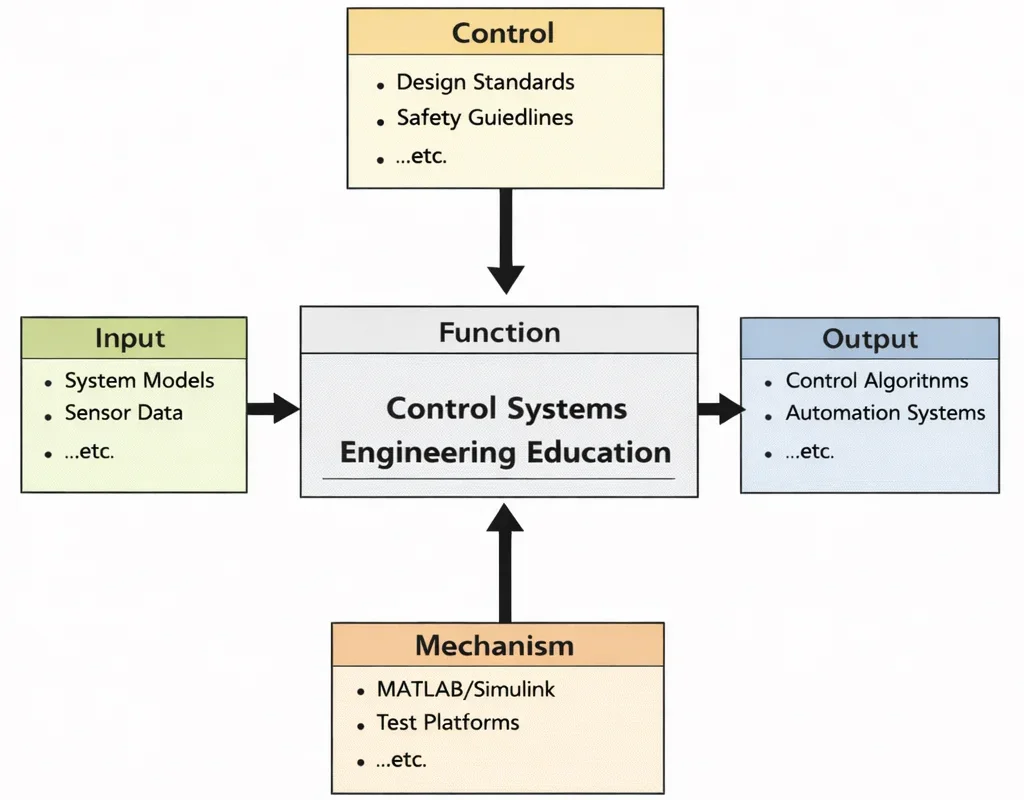
Prepare for University Studies & Career Advancement

Control Systems Engineering

Control Systems Engineering Education is, at its heart, the art of teaching systems to behave—calmly, safely, and on purpose—when the real world refuses to be predictable. In the diagram, Inputs, such as models and sensor data, represent the raw “evidence” of how a system moves, drifts, and responds. Controls, such as standards and safety rules, act like the guardrails of good engineering judgment, ensuring designs do more than work in theory—they work responsibly. The Mechanisms, including simulation tools and test platforms, provide the workshop where ideas can be built, stressed, and refined without guesswork. From this disciplined pathway come the Outputs: algorithms and automation solutions that translate mathematics into behavior—systems that can track, stabilize, reject disturbances, and ultimately earn trust in everything from machines and vehicles to infrastructure and modern devices.

Figure 1: IDEF0 architectural model of Control Systems Engineering Education: converting mathematical models and telemetry into validated closed-loop feedback algorithms.

Control Systems Engineering is a foundational discipline that underpins automation, robotics, aerospace systems, and advanced electronics. As a branch of Electrical and Electronic Engineering, it focuses on the modeling, analysis, and design of systems that respond predictably to inputs. These systems range from mechanical feedback loops to smart electrical grids, forming the core of many modern technologies.

Core concepts in control systems are enriched by developments in Electronics Engineering and the miniaturization of circuits through Embedded Systems and Microelectronics. These advancements allow for real-time control in devices ranging from wearable health monitors to autonomous vehicles. Control strategies also depend on accurate Instrumentation and Measurement, which ensures the feedback needed to maintain stability and performance.

With the proliferation of interconnected devices, Control Systems Engineering increasingly interfaces with the Internet of Things (IoT) and Smart Technologies. These technologies enable adaptive behavior in distributed networks such as traffic control systems and smart manufacturing lines. In energy infrastructure, control systems are essential in the regulation of Power Systems Engineering and in maximizing the efficiency of Renewable Energy and Energy Storage.

Precision control is critical in emerging areas such as Quantum Electronics, where maintaining coherence in quantum states is vital. Similarly, Robotics and Automation in E&E rely on carefully tuned control algorithms for locomotion, manipulation, and autonomous decision-making. Enhancing these capabilities requires integrated knowledge from Signal Processing for filtering noise and interpreting sensor data.

Control systems also play a vital role in sectors related to health and environment. For instance, Biomedical Electronics employs control logic in devices like pacemakers and insulin pumps. In environmental sectors, systems are designed to regulate conditions in Air Quality Engineering and manage resources through Water Resources Engineering. Accurate data collection from Environmental Monitoring and Data Analysis helps automate interventions and maintain compliance with Environmental Policy and Management.

Control techniques also support urban sustainability through Green Building and Sustainable Design and the coordination of circular production systems in Industrial Ecology and Circular Economy. Whether in energy grid balancing, industrial process optimization, or Waste Management Engineering, control systems enable efficiency and resilience. Students can also explore related innovations in Renewable Energy Systems Engineering and Industrial and Manufacturing Technologies.

As students delve into this field, they gain a multidisciplinary perspective that links theory and application—from dynamic system modeling and PID controllers to AI-enhanced predictive systems. Control Systems Engineering is an ideal path for those seeking to design intelligent, responsive technologies that shape our increasingly automated and sustainable world.

Interactive PID Closed-Loop Step Response Simulator

Adjust the Proportional ($K_p$), Integral ($K_i$), and Derivative ($K_d$) gains to observe real-time second-order system response $y(t)$ to a unit step input. Evaluate transient peak overshoot ($M_p$), rise time ($T_r$), settling time ($T_s$), and steady-state error ($e_{ss}$).

Proportional Gain $K_p$: 2.0

Integral Gain $K_i$: 0.5

Derivative Gain $K_d$: 1.0

System Status: Stable Closed-Loop

Peak Overshoot: 12.4%

Steady-State Value: 1.00

Simulation runtime engine: Prep4Uni.Online Control Systems Engineering Hub

Control engineer studying holographic telemetry dashboards, digital twin system model, and an articulated multi-axis industrial robotic manipulator

Figure 2: Control Systems Engineering — using feedback, sensors, and algorithms to keep machines stable, efficient, and safe.

The illustration shows a modern industrial workspace where a control engineer stands with folded arms, analysing a floating interface of graphs, dials, and system icons. A bright, projected platform on the table suggests a digital twin view of a controlled process, while nearby robotic equipment and factory piping hint at real-world automation. The layered readouts evoke feedback loops, tuning, monitoring, and AI-assisted optimisation—capturing how control systems coordinate complex machines and processes in manufacturing and beyond.

Control Systems Engineering: Feedback, Stability, and System Regulation

Electrical & Electronic Engineering – Overview

Establishes the foundational discipline governing electronic networks, energy conversion, and signal acquisition that underpin all physical control mechanisms.

Control Systems Engineering (Current Topic)

Designs feedback mechanisms, stability criteria, and dynamic compensators to ensure accurate, repeatable system regulation under external disturbances.

Signal Processing

Filters environmental noise and conditions raw sensor telemetry, delivering clean state estimates into closed-loop feedback algorithms.

Instrumentation & Measurement

Provides physical-to-electrical transduction, measuring key system variables (temperature, pressure, speed) needed for precise controller action.

Embedded Systems & Microelectronics

Hosts discrete-time control routines within microcontrollers, DSPs, and FPGAs for real-time execution in compact physical hardware.

Robotics & Automation in EE

Directs multi-axis joint trajectory, balance, and spatial navigation by coordinating motor actuation via robust, adaptive control loops.

Power Systems Engineering

Utilizes automated voltage regulation and automatic generation control to stabilize grid frequency across large power generation grids.

Renewable Energy & Energy Storage

Implements Maximum Power Point Tracking (MPPT) and battery charge balancing algorithms to optimize fluctuating green energy supplies.

Communication Engineering

Transmits feedback telemetry and distributed control commands securely over wired and wireless networks with minimal latency.

IoT & Smart Technologies

Enables cloud-edge control loops, allowing smart municipal systems and factory IoT networks to adjust operational states dynamically.

Electronics Engineering

Designs the operational amplifiers, analog filters, and power switching transistors required to drive physical actuators efficiently.

Quantum Electronics

Applies precise electro-magnetic control pulse sequences to preserve qubit state coherence and manage quantum decoherence limits.

Biomedical Electronics

Incorporates closed-loop regulation into pacemakers, automated insulin delivery, and artificial organ support systems for biological stability.

Core Concepts in Control Systems Engineering

Control systems engineering lies at the heart of modern automation and intelligent system design. It provides the theoretical foundations and practical methodologies needed to make machines and processes respond predictably, efficiently, and safely. This expanded overview explores the key concepts, methodologies, and real-world implications of control systems engineering, highlighting its importance across industries that rely on precision and reliability.

Control System Types
- Open-Loop Control Systems: These systems operate without feedback—the control action is independent of the output. A classic example is a basic washing machine timer: it runs for a preset time regardless of load size or cleaning effectiveness. Although simple and cost-effective, open-loop systems can be inaccurate when process parameters change.
- Closed-Loop (Feedback) Control Systems: In these systems, the output is continuously monitored and fed back to adjust control actions. This feedback allows self-correction. For example, a thermostat regulates room temperature by switching heating on or off depending on the measured ambient temperature. Closed-loop systems offer higher precision and robustness against disturbances.
Understanding the distinction between open- and closed-loop systems is foundational—choosing the right structure underpins everything from household appliances to advanced aerospace applications.
System Dynamics and Modeling Control engineers must understand how processes respond over time. This requires constructing mathematical models using techniques such as differential equations, transfer functions, or state-space representations. For example, modeling a motor could involve parameters like inertia, friction, and torque. Engineers also rely on system identification—experimental methods to infer dynamic behavior from test data. Accurate models are essential for controller design, stability assessment, and simulation-based testing.
Stability Analysis Stability ensures systems behave predictably and do not exhibit runaway or oscillatory behavior. Engineers use tools such as:
- Routh–Hurwitz Criterion: An algebraic method to determine system stability from the coefficients of the characteristic equation without explicitly computing roots.
- Nyquist Plots: Frequency-domain polar plots that reveal how encirclements of the $-1 + j0$ point dictate closed-loop stability margins.
- Lyapunov Stability Analysis: A rigorous energy-like state-space framework essential for analyzing global stability in nonlinear autonomous systems.
Ensuring stability is a central duty of control engineers—it underpins safe and dependable operation in systems from power grids to medical devices.
Control Strategies
- Proportional-Integral-Derivative (PID) Control: A widely used controller type that corrects the present error (Proportional), accumulates past errors (Integral), and anticipates future error trends (Derivative). PID controllers are prevalent in industrial automation, robotics, HVAC systems, and instrumentation.
- State-Space Control: This framework represents dynamic systems through first-order matrix differential equations, enabling full-state feedback pole placement, linear quadratic regulators (LQR), and Kalman filter state estimators.
- Adaptive Control: These controllers adjust their own parameters in real time, maintaining performance in the face of changing dynamics—used in aerospace control and precision manufacturing.
- Robust Control: Designed to maintain performance despite uncertainty—such as parameter variations, external disturbances, or unmodeled high-frequency dynamics. Techniques like $H_\infty$ synthesis and $\mu$-analysis are central to safety-critical systems.
Each control strategy offers trade-offs in simplicity, performance, and robustness. The choice depends on system requirements and operating environments.
Sensors and Actuators Sensors gather data about the system’s state—e.g., temperature via thermocouples, pressure via strain gauges, or position via optical encoders. Actuators (motors, valves, hydraulic pistons) convert control commands into physical actions. Engineers must consider factors like sensor accuracy, dynamic range, and latency, along with actuator response speed and power saturation limits. Proper integration ensures reliable feedback and precise control.
Digital Control Modern control systems are predominantly digital, implemented using microcontrollers, programmable logic controllers (PLCs), field-programmable gate arrays (FPGAs), or digital signal processors (DSPs). Digital systems offer programmability, robustness to noise, and advanced algorithm support, but introduce complexities like quantization error, finite-wordlength effects, and sampling delays. Engineers design around these constraints using bilinear Tustin transformations and discrete z-domain analysis to ensure stable performance.

Applications of Control Systems Engineering

Control systems engineering is foundational to modern automation, enabling machines, processes, and infrastructures to perform reliably, adaptively, and with precision. Its applications span robotics, manufacturing, aerospace, automotive systems, energy management, healthcare, smart infrastructure, and defense. Each domain relies on advanced sensing, real‑time feedback, intelligent control strategies, and robust hardware to achieve performance, efficiency, safety, and autonomy. The sections below explore these applications in depth, highlighting how control engineering transforms industry and society.

Robotics Control systems enable robots to perform tasks autonomously and with precision across diverse environments.
- Motion Control: Feedback loops, servo motors, and trajectory planning ensure smooth, accurate movements in robotic arms used for assembly, welding, and material handling.
- Path Planning and Navigation: Localization, SLAM (Simultaneous Localization and Mapping), and sensor fusion allow mobile robots and aerial drones to navigate complex indoor/outdoor environments while avoiding obstacles.
- Human‑Robot Interaction: Safety‑centric control enables cobots—robots working alongside humans—to adjust speed or path when humans approach, using force sensors and collision‑detection algorithms.
Manufacturing and Automation Industrial processes rely on control systems for consistency, quality, and efficiency.
- Process Control: PID loops regulate pressure, temperature, and flow in chemical plants, refineries, food production, and pharmaceutical processing.
- Assembly Lines: Coordinated PLCs (Programmable Logic Controllers) and robotic cells automate sequential tasks at high speed, ensuring precise timing and synchronized operation.
- Quality Control: Cameras, laser scanners, and statistical process control systems detect defects in real time and adjust parameters to ensure consistent product quality.
Aerospace Systems Aircraft and spacecraft depend on advanced control systems for stability, navigation, and autonomous operation.
- Flight Control: Autopilots, fly‑by‑wire systems, and attitude control systems enable precise maneuvers, path tracking, and turbulence compensation.
- Space Exploration: Reaction wheels, thrusters, and guidance controllers manage satellite orientation, orbital maneuvers, and robotic operations on planetary missions.
- Unmanned Aerial Vehicles (UAVs): Controllers manage flight stability, mission planning, obstacle avoidance, and adaptive behavior in real time.
Automotive Engineering Vehicles increasingly rely on embedded control systems for safety, comfort, and autonomy.
- Cruise Control and Adaptive Cruise Control: These systems use feedback from speed sensors and radar/vision systems to maintain set speed or adjust based on traffic flow.
- Electric and Autonomous Vehicles: Motor control algorithms regulate torque, manage battery usage, and support automated navigation systems.
- Stability Control Systems: Electronic Stability Control and anti‑skid systems adjust braking and torque in milliseconds to prevent loss of control.
Energy Systems Efficient energy generation and distribution depend on intelligent control.
- Power Grid Management: Controllers balance generation, demand, and frequency across transformers, generators, and substations.
- Renewable Energy Integration: Control algorithms maximize power output from wind turbines, solar panels, and battery storage while stabilizing grid interactions.
- Smart Grids: Systems use sensors, bidirectional control, and load forecasting to optimize distribution and minimize losses.
Healthcare and Biomedical Systems Critical medical devices rely on responsive, fail-safe control systems.
- Medical Devices: Ventilators, infusion pumps, and dialysis machines use closed‑loop feedback to regulate flow, pressure, and dosage.
- Prosthetics and Exoskeletons: Actuator feedback in response to neural or muscle signals enables intuitive movement and rehabilitation support.
- Imaging Systems: MRI and CT scanners rely on precise electromagnetic and hydraulic control for accurate scanning and safe operation.
Infrastructure and Building Automation Intelligent building systems increase comfort, safety, and energy efficiency.
- HVAC Systems: Feedback-controlled heating, ventilation, and cooling systems maintain indoor climate while minimizing energy consumption.
- Smart Buildings: Networked sensors and controllers manage lighting, security, occupancy detection, and resource monitoring.
- Elevators and Escalators: Speed, position, and load sensors ensure safe, smooth, and efficient vertical transportation.
Defense and Military Applications Control engineering ensures accuracy, resilience, and autonomy in tactical systems.
- Guided Missiles: Inertial sensors, GPS guidance, and dynamic control loops correct trajectory for precision targeting.
- Radar and Tracking Systems: Real-time signal processing and antenna steering optimize detection and tracking of airborne and maritime objects.
- Autonomous Combat Systems: Self‑navigating unmanned ground and aerial vehicles process sensor data to make mission-level decisions.

Contemporary Computational Paradigms in Modern Control

Modern control systems increasingly confront complex multi-physics coupling, unmodeled environmental dynamics, and strict millisecond-scale execution limits. Contemporary computational frameworks bridge classical feedback theory with data-driven neural operators and geometric estimation:

Physics-Informed Neural Networks (PINNs) in Optimal Control: By embedding Hamilton-Jacobi-Bellman (HJB) partial differential equations directly into the training loss: $$\mathcal{L}_{\text{total}} = \mathcal{L}_{\text{data}} + \lambda_{\text{HJB}} \left\| \frac{\partial V(\mathbf{x})}{\partial t} + \min_{\mathbf{u} \in \mathcal{U}} \left\{ \nabla V(\mathbf{x}) \cdot f(\mathbf{x}, \mathbf{u}) + \mathcal{C}(\mathbf{x}, \mathbf{u}) \right\} \right\|^2$$ PINNs overcome the "curse of dimensionality" in dynamic programming, enabling continuous-time value function $V(\mathbf{x})$ estimation and real-time nonlinear optimal control feedback without grid discretization.
DeepONets & Neural Operators for Model Predictive Control (MPC): Standard online MPC solves an open-loop quadratic program (QP) at every sampling step. For micro-second robotic actuators and hypersonic flight controllers, DeepONets and Fourier Neural Operators (FNOs) learn the parametric solution map from current plant states $\mathbf{x}_0$ directly to the optimal control sequence $\mathbf{u}^*(t)$, reducing online solver time from milliseconds to microseconds.
Invariant Extended Kalman Filters (IEKF) on Lie Groups: In aerial robotics, aerospace navigation, and legged locomotion, state estimation errors cause severe control degradation. IEKF formulates the state observer over the matrix Lie group $SE_2(3)$, guaranteeing that filter error dynamics remain invariant to trajectory deviations and eliminating coordinate singularities.
Real-Time Digital Twins & Automated FDIR: Industrial plant digital twins run synchronized state observers alongside physical hardware. By running continuous Model-Based Fault Detection, Isolation, and Recovery (FDIR), the supervisory engine detects actuator bias, sensor freeze, or pipe leakage, switching to redundant control modes within milliseconds.

Challenges in Control Systems Engineering

Control systems engineering is deeply embedded in critical and complex infrastructures—from aerospace and automotive systems to industrial automation and healthcare devices. Despite its wide-reaching influence, the field continues to grapple with multifaceted challenges that reflect the demands of modern technology and societal expectations. This expanded overview delves into the nuanced hurdles facing control engineers today:

System Complexity and Multi-Physics CouplingContemporary control applications are composed of numerous interconnected subsystems—mechanical, electrical, hydraulic, thermal, and software—all interacting in dynamic ways. Modeling these components accurately requires high-fidelity representations such as nonlinear state-space models, hybrid automata, and multi-domain simulations. Engineers often resort to balanced truncation model order reduction (MOR) to preserve controllability and observability Gramians while reducing computational burden. Co-simulation frameworks allow for testing multi-physics interactions, ensuring modular designs and system-wide consistency across domains. Ensuring coherence in control design under such complexity demands modular architectures, hierarchical control layers, and rigorous integration testing.
Uncertainty, Stochastic Noise, and Disturbance AttenuationReal-world systems are subject to varying parameters—Coulomb friction, mechanical backlash, load inertia variations, wear, temperature—as well as unmodeled high-frequency structural resonances. Traditional control methods like linear PID may fail under these conditions. Robust control designs utilizing $H_\infty$ loop shaping and structured singular value ($\mu$) analysis provide strict performance guarantees under norm-bounded plant perturbations $\|\Delta(s)\|_\infty \lt 1$. Stochastic methods such as Extended Kalman Filters and unscented transforms enhance resilience to measurement noise, while active fault-tolerant architectures compensate for component wear dynamically.
Safety, Actuator Saturation, and Anti-Windup BoundariesHigh-stakes applications—like aerospace flight decks, nuclear reactivity rods, and surgical robotics—demand system designs that fail safely and reliably. In physical implementations, actuators have finite force, torque, and slew rate limits. When a controller commands effort beyond these physical ceilings, the feedback loop opens, leading to integral windup, large phase delays, and catastrophic overshoot. Engineers implement conditioned integration anti-windup circuits, watchdog hardware monitors, and formal reachability verification to mathematically prove that trajectories never cross unsafe barrier envelopes.
Integration with Emerging Technologies and CPS CybersecurityIncorporating AI, IoT, and machine learning into control systems offers adaptability and contextual awareness but introduces non-deterministic unpredictability. Learning-based controllers must be validated through formal contraction analysis and adversarial stress testing. In Cyber-Physical Systems (CPS), networked feedback loops share industrial Ethernet or wireless channels, introducing packet dropouts, variable transmission delay (jitter), and susceptibility to false-data-injection (FDI) cyber-attacks on sensor measurements, requiring hardware roots-of-trust and secure state estimators.
Deterministic Real-Time Timing Constraints and Computational LatencyMany control applications—autonomous vehicle collision avoidance, active magnetic bearings, and quadrotor attitude stabilization—require control loop update rates exceeding $1\,\text{kHz}$ ($\Delta t \lt 1\,\text{ms}$). These systems must execute sensing, state estimation, optimization, and pulse-width modulation (PWM) actuation deterministically without execution jitter. Engineers deploy real-time operating systems (RTOS) with pre-emptive scheduling and synthesize hardware control pipelines directly onto FPGA fabric.

Future Trends in Control Systems Engineering

Control systems engineering is entering a transformative era driven by advances in artificial intelligence, digital technologies, and environmental imperatives. These trends are redefining how engineers design, monitor, and deploy control strategies across industries—from manufacturing floors to urban infrastructure. The following sections explore six major emerging trends, revealing their technological depth, real-world applications, and broader significance for a smarter, sustainable future.

AI and Physics-Informed Learning Control
- AI-powered controllers are being developed to anticipate system behavior, identify anomalies, and adjust in real time—improving performance and fault tolerance beyond what traditional PID or model-based controllers can achieve.
- Reinforcement learning enables autonomous agents to learn optimal control policies through trial and error. Embedded with Lyapunov barrier functions, safe reinforcement learning guarantees asymptotic stability during the exploration process across autonomous vehicles, robotic surgery, and adaptive flight control.
Decentralized and Distributed Consensus Control In large-scale and geographically dispersed systems—like smart grids, multi-agent drone swarms, and urban water networks—centralized control cannot scale. Distributed control architectures break the system into semi-autonomous nodes that exchange local telemetry over communication graphs and reach mathematical consensus via distributed alternating direction method of multipliers (ADMM).
Digital Twins and Real-Time Predictive Simulation Digital twins are dynamic, real-time virtual replicas of physical systems. They integrate sensor data, finite-element models, and simulation engines to monitor degradation, run predictive maintenance analytics, and evaluate control parameter adjustments without disrupting operational plants.
Advanced Industrial IoT Sensing and Edge Control The proliferation of high-precision MEMS sensors and edge computing silicon enables localized condition monitoring and sub-millisecond control actions. Smart sensor nodes preprocess raw vibration and temperature data directly at the bearing housing, executing edge filtering and local disturbance rejection.
Quantum State Control and Error Correction As quantum computing advances, control engineering is fundamental to managing quantum dynamics. Optimal pulse shaping algorithms (e.g., GRAPE - GRadient Ascent Pulse Engineering) manipulate microwave and laser waveforms to steer qubit states along Bloch spheres with high gate fidelities, actively suppressing environmental decoherence.
Sustainable and Carbon-Optimized Green Control Environmental sustainability is increasingly embedded in control objective functions. Engineers design predictive building HVAC controllers that balance thermal comfort against real-time grid carbon intensity tariffs, while power plant governors modulate generation ramping to maximize green energy penetration.

Worked Numerical Application: Second-Order Servomechanism & PID Controller Synthesis

Engineering Calculation: Closed-Loop Pole Placement & PD Damping Design

Problem Formulation: An industrial DC motor positioning table is described by the open-loop transfer function: $$G(s) = \frac{10}{s(s + 2)}$$ The positioning system operates under unity negative feedback. To meet strict precision manufacturing tolerances, the closed-loop step response must achieve: (1) A maximum percentage overshoot $M_p \le 4.32\%$; (2) A $2\%$ settling time $T_s \le 1.0\,\text{second}$. Determine whether uncompensated proportional control can meet these specifications. If not, design a Proportional-Derivative (PD) controller $G_c(s) = K_p + K_d s$ to place the closed-loop poles at the required design location.

Analytical Derivation & Step-by-Step Calculations:

Step 1: Determine Required Damping Ratio ($\zeta$) and Natural Frequency ($\omega_n$):

From the overshoot specification:

$$M_p = \exp\left( \frac{-\zeta \pi}{\sqrt{1 - \zeta^2}} \right) \le 0.0432 \quad \Rightarrow \quad \frac{\zeta \pi}{\sqrt{1 - \zeta^2}} = -\ln(0.0432) \approx 3.1419$$ $$\frac{\zeta^2}{1 - \zeta^2} = \left(\frac{3.1419}{\pi}\right)^2 \approx 1.0 \quad \Rightarrow \quad \zeta^2 = 0.5 \quad \Rightarrow \quad \mathbf{\zeta = \frac{1}{\sqrt{2}} \approx 0.7071}$$

From the $2\%$ settling time specification ($T_s \approx \frac{4}{\zeta \omega_n}$):

$$T_s = \frac{4}{\zeta \omega_n} \le 1.0\,\text{s} \quad \Rightarrow \quad \zeta \omega_n \ge 4.0 \quad \Rightarrow \quad \omega_n \ge \frac{4.0}{0.7071} \approx \mathbf{5.657\,\text{rad/s}}$$

Select the minimum natural frequency $\omega_n = 5.657\,\text{rad/s}$. The desired characteristic equation is:

$$\Delta_{\text{desired}}(s) = s^2 + 2\zeta\omega_n s + \omega_n^2 = s^2 + 2(4.0)s + (5.657)^2 = \mathbf{s^2 + 8.0s + 32.0 = 0}$$

Step 2: Evaluate Proportional Control Alone ($G_c(s) = K_p$):

With pure proportional gain, the characteristic equation is $1 + K_p G(s) = 0$:

$$s(s + 2) + 10 K_p = s^2 + 2s + 10 K_p = 0$$

Comparing with standard form: $2\zeta\omega_n = 2 \Rightarrow \zeta\omega_n = 1.0$.
Thus, settling time with pure proportional control is fixed at $T_s = \frac{4}{1.0} = \mathbf{4.0\,\text{seconds}}$, regardless of the choice of $K_p$. Proportional gain alone cannot speed up the system to meet $T_s \le 1.0\,\text{s}$.

Step 3: Synthesize PD Controller Gains ($K_p$ and $K_d$):

With a PD compensator $G_c(s) = K_p + K_d s$, the closed-loop characteristic equation is:

$$1 + G_c(s) G(s) = 1 + (K_p + K_d s) \frac{10}{s(s + 2)} = 0$$ $$s(s + 2) + 10(K_p + K_d s) = s^2 + (2 + 10 K_d)s + 10 K_p = 0$$

Equating coefficients to the desired characteristic equation $s^2 + 8.0s + 32.0 = 0$:

$$2 + 10 K_d = 8.0 \quad \Rightarrow \quad 10 K_d = 6.0 \quad \Rightarrow \quad \mathbf{K_d = 0.60\,\text{s}}$$ $$10 K_p = 32.0 \quad \Rightarrow \quad \mathbf{K_p = 3.20}$$

Physical & Engineering Takeaways: The uncompensated motor suffers from fixed velocity damping ($B/J = 2$), which constrains the real part of the system poles to $-1$. Adding derivative feedback ($K_d = 0.60$) introduces artificial active damping via back-EMF feedback emulation, quadrupling the pole real part to $-4$ and cutting the settling time from $4.0\,\text{s}$ down to $1.0\,\text{s}$ while maintaining low overshoot ($4.32\%$).

Systems Engineering Architecture: Trade-Off Analysis

Designing dynamic feedback control systems involves balancing competing physical, computational, and algorithmic requirements. The following matrix illustrates key engineering compromises in controller selection:

Control Strategy	Architectural Paradigm	Favorable Attributes (+)	Compromised Metrics (−)	System Mitigation Strategy
Classical PID	Error-driven linear feedback (SISO)	Computationally lightweight; model-free heuristic tuning; simple implementation on 8-bit microcontrollers.	Cannot handle multivariable cross-coupling; poor handling of hard state/actuator constraints; susceptible to derivative noise.	Implement low-pass derivative filters and anti-windup clamping schemes.
Model Predictive Control (MPC)	Receding horizon online optimization	Handles multivariable MIMO systems; incorporates state, input, and slew-rate constraints directly into quadratic cost.	High computational overhead; requires high-throughput processors; potential solver failure if non-convex.	Explicit MPC (precomputed look-up tables) or neural operator surrogates (DeepONets).
$H_\infty$ Robust Control	Worst-case frequency-domain optimization	Guaranteed stability and performance under norm-bounded plant variations and high-frequency modeling errors.	Conservative transient performance; high-order controller transfer functions that complicate embedded implementation.	Hankel norm model order reduction to eliminate unobservable controller states.
Sliding Mode Control (SMC)	Variable structure nonlinear control	Completely insensitive to matched internal uncertainties and external disturbances once on the sliding manifold.	High-frequency control chattering that excites mechanical resonances and accelerates actuator wear.	Boundary layer continuous approximation (saturation function) or higher-order super-twisting SMC.

Societal and Economic Impact

Control systems engineering has emerged as a key driver of societal progress and economic vitality. By embedding advanced automation, intelligent decision-making, and precise control into a wide array of systems, control engineering not only boosts efficiency and safety, but also sparks innovation, fosters employment, and enhances global competitiveness. Here’s an in-depth analysis of its profound impact:

Enhanced Efficiency: Automation and control systems reduce operational costs and resource consumption in industries. From manufacturing plants and energy facilities to transportation networks and agricultural operations, control systems underpin streamlined processes. Automated assembly lines regulated by PID controllers and robotics optimize cycle times and throughput, while reducing waste and increasing precision. Smart energy management systems dynamically balance power loads and reduce peak demand, resulting in significant energy savings and cost reductions. In agriculture, sensor-driven irrigation controllers ensure optimal watering schedules, conserving water while maximizing crop yields. These systems leverage real-time data, predictive analytics, and adaptive algorithms to continuously optimize performance, delivering sustained operational excellence.
Improved Safety: Systems designed with robust control mechanisms enhance safety in applications like transportation and healthcare. Safety-critical control applications save lives and minimize risks. In transportation, automotive stability control, anti-lock braking, and flight control systems maintain safe operation under adverse conditions or failures. In healthcare, ventilators, infusion pumps, and surgical robots rely on precise control loops to deliver critical therapies reliably and safely. Redundant sensor arrays, fail-safe logic, and real-time monitoring ensure that even in fault conditions, systems enter safe states rather than fail catastrophically. Formal methods and certification standards further guarantee reliability in mission-critical environments.
Job Creation: The growth of control systems engineering drives demand for skilled professionals in research, development, and implementation. Demand for specialists in control theory, embedded design, robotics, and automation has soared across industries. Engineers design and validate control software, integrate sensors and actuators, and develop custom hardware solutions. Technicians install and maintain control systems in industrial plants, while researchers push the boundaries of AI-driven and quantum-based control. In academia, professionals train the next generation through university programs and workshops, while policymakers and consultants guide technology adoption. This creates a wide ecosystem of careers in engineering, IT, research, consultancy, and vocational training.
Global Competitiveness: Nations and companies investing in advanced control systems gain a competitive edge in technology-driven markets. Countries that lead in automation, smart infrastructure, and advanced manufacturing are better positioned for economic growth. Companies that deploy sophisticated control solutions produce higher-quality outputs more efficiently, giving them an edge in global sectors like automotive, aerospace, energy, electronics, and defence. Investment in national initiatives—such as Industry 4.0, smart cities, and renewable energy integration—enhances productivity and stimulates innovation ecosystems. Cross-border collaboration and trade in control technologies further reinforce innovation cycles and economic resilience.

Why Study Control Systems Engineering

Understanding Dynamic Systems and Feedback: Control systems engineering focuses on how systems respond to inputs and maintain stability. Students learn about feedback loops, transfer functions, and system behavior. This understanding is key to designing reliable systems.

Designing Automated and Responsive Systems: Students study how to design systems that regulate processes automatically. Applications include cruise control, robotics, HVAC, and industrial automation. These designs improve efficiency, accuracy, and safety.

Mathematical Modeling and Simulation: The course introduces tools like MATLAB/Simulink for modeling system dynamics. Students learn how to simulate responses and optimize control strategies. This prepares them to troubleshoot and refine complex systems.

Applications in Robotics and Aerospace: Control systems are vital in robotics, drones, aircraft, and spacecraft. Students explore how to manage orientation, speed, and navigation. These skills are essential for advanced technological development.

Cross-Disciplinary Relevance and Innovation: Control engineering intersects with mechanical, electrical, and software fields. Students develop versatile skills applicable across industries. This opens doors to careers in automation, manufacturing, and research.

Control Systems Engineering Conclusion

Control systems engineering is a cornerstone of modern technological advancement, enabling automation, efficiency, and innovation across industries. From aerospace to automotive, from industrial manufacturing to biomedical systems, control engineering ensures that complex processes function with precision, responsiveness, and stability. By designing feedback loops, optimizing system dynamics, and implementing intelligent control algorithms, engineers in this field create the invisible infrastructure that keeps our machines, networks, and processes running smoothly.

As automation continues to transform traditional workflows, control systems have become increasingly sophisticated—integrating sensors, actuators, and real-time data analytics to make autonomous decisions. These systems not only enhance productivity but also ensure safety, reduce energy consumption, and improve system longevity. For example, in smart factories, adaptive control systems can automatically adjust machinery settings in response to sensor inputs, reducing waste and increasing yield.

The impact of control systems is not confined to industry. In everyday life, we rely on them in household appliances, climate control systems, elevators, and even smartphones. In transportation, they are at the heart of anti-lock braking systems, cruise control, and autonomous driving technologies. In healthcare, control systems govern life-saving devices such as ventilators, infusion pumps, and robotic surgical tools—demonstrating their vital role in both critical and routine functions.

Looking to the future, control systems engineering is set to play a pivotal role in emerging technologies. Integration with artificial intelligence and machine learning allows for predictive control models that can adapt to complex and changing environments. Cyber-physical systems and digital twins are extending control paradigms beyond traditional boundaries, enabling real-time monitoring and simulation of entire industrial plants or cities. In power systems, advanced control strategies are crucial for managing decentralized energy sources, including solar, wind, and battery storage, ensuring grid stability and optimizing resource use.

Moreover, control systems are central to sustainability and environmental stewardship. In green buildings and smart cities, intelligent HVAC and lighting systems respond dynamically to occupancy and ambient conditions, drastically reducing energy waste. Precision agriculture leverages sensor-guided control systems to optimize irrigation, fertilization, and harvesting—boosting productivity while conserving resources. These applications highlight how control engineering contributes directly to sustainable development goals.

One of the most exciting frontiers is in autonomous systems—drones, robots, and self-driving vehicles—where control engineering ensures reliable navigation, decision-making, and safety in real-world environments. These systems must process vast streams of data, account for uncertainties, and respond in milliseconds, requiring robust and fault-tolerant control architectures.

Education and research in control systems are also evolving, with students learning through simulation environments, hardware-in-the-loop systems, and collaborative robotics. Interdisciplinary curricula now blend control theory with computer science, signal processing, and system engineering to prepare the next generation for a connected, autonomous, and intelligent world. Open-source platforms and cloud-based tools are democratizing access to advanced control design, empowering engineers across the globe.

Ultimately, control systems engineering is more than a field of technical practice—it is a driving force behind the automation and intelligence embedded in our modern infrastructure. As the demands on systems grow in complexity, control engineers will continue to deliver innovative solutions that bridge the gap between theory and application. Whether addressing climate change, ensuring the reliability of mission-critical operations, or enhancing daily life, the discipline will remain at the heart of our technological evolution—shaping a smarter, safer, and more responsive future for all.

Frequently Asked Questions

1. What does a control engineer actually do?

Control engineers design systems that automatically regulate variables such as speed, temperature, position, or pressure. They decide how to sense what is happening, how to compare it with a desired target, and how to move actuators so that the system behaves in a safe, stable, and efficient way.

2. Why is feedback control used instead of just “setting” an input once?

Real systems face disturbances, wear, and modelling inaccuracies. If you simply set an input once (open-loop control), the output will drift when conditions change. Feedback control continually measures the output and adjusts the input, keeping the system close to its setpoint despite changing loads or environments.

3. What makes stability such a big concern in control systems?

A system can be very fast or accurate, but if it is unstable, small disturbances can grow into large oscillations or even physical damage. Stability is the foundation: only after ensuring that responses remain bounded can engineers focus on improving speed, accuracy, and robustness.

4. Where do we see PID controllers in everyday life?

PID controllers appear in many familiar applications: cruise control in cars, temperature control in ovens and air conditioners, speed control in motors, and level control in tanks. They are popular because a single structure can be tuned to work well for many different processes.

5. Why do control engineers use transfer functions and Bode plots?

Transfer functions and Bode plots make it easier to understand how a system responds across different frequencies. They show where the system amplifies or attenuates signals and reveal how close it is to instability. This helps engineers tune controllers and compensators without trial-and-error alone.

6. What is the difference between classical control and modern state-space methods?

Classical control often focuses on single-input, single-output systems using transfer functions and frequency-domain tools. Modern control uses state-space models and matrix methods, which naturally handle multiple inputs and outputs, constraints, and advanced strategies like optimal or robust control.

7. What does a compensator do in a control loop?

A compensator is an extra dynamic block added to the loop to “shape” the system’s behaviour. With suitable design, a compensator can speed up the response, reduce overshoot, improve steady-state accuracy, and give the system more comfortable stability margins.

8. Why are advanced methods like model predictive control (MPC) attracting attention?

Modern processes often have multiple interacting variables and strict constraints on safety or energy use. MPC looks ahead in time using a model of the plant and computes control actions that optimise performance while respecting constraints. This makes it attractive for chemical plants, energy systems, and autonomous vehicles where simple PID control may struggle.

9. How do control systems cope with nonlinearity and uncertain parameters?

Engineers use strategies such as gain scheduling, robust control, and adaptive control. These approaches either design controllers that tolerate variation, switch between different controller settings for different operating regions, or update controller parameters online as the system behaviour changes.

10. How is control systems engineering linked to robotics and automation?

Robotics and automation rely on control systems to move actuators precisely, follow paths, balance robots, and coordinate multiple axes or machines. Without well-designed control algorithms, robots would be jerky, inaccurate, and unsafe, and automated production lines would not achieve the required throughput or quality.

Control Systems Engineering Practice Module

Section 1: Foundational Review Questions

1. What distinguishes open-loop control from closed-loop (feedback) control, and why is feedback often essential in engineering applications?

Answer: In an open-loop system, the controller sends commands based only on a prescribed input or schedule and does not measure the actual output. As a result, it cannot correct for disturbances, parameter changes or modelling errors. In a closed-loop system, sensors measure the output and feed it back to the controller, which continuously adjusts the input to reduce the error between the measured value and the desired setpoint. This feedback mechanism is essential in many engineering applications—such as cruise control, industrial temperature regulation or motor speed control—because it provides automatic correction and keeps performance acceptable under varying operating conditions.

2. Why is stability so crucial in control systems, and how do engineers assess it?

Answer: Stability determines whether a system’s response to inputs or disturbances remains bounded and well-behaved. An unstable system may exhibit growing oscillations or diverging outputs, which can damage equipment or endanger safety. Engineers assess stability using mathematical and graphical tools, such as location of poles in the complex plane, the Routh–Hurwitz criterion, Nyquist plots and Bode plots. These methods reveal whether the closed-loop poles lie in stable regions and how close the system is to instability. If necessary, designers adjust controller parameters or introduce compensators to move the poles to more desirable locations.

3. How do PID controllers function, and what roles do the proportional, integral, and derivative terms play?

Answer: A PID controller generates its output by combining three actions based on the control error (the difference between setpoint and measured output). The proportional term responds to the current error, providing an immediate corrective action. The integral term accumulates past error over time, driving the steady-state error towards zero. The derivative term anticipates the future trend of the error by responding to its rate of change, helping to damp oscillations and improve transient performance. By tuning the three gains, engineers can shape response speed, overshoot and accuracy for a wide variety of processes.

4. What is the role of transfer functions in classical control theory, and how do they simplify system analysis?

Answer: Transfer functions describe the input–output relationship of linear time-invariant systems in the Laplace domain as ratios of polynomials in the complex variable $s$. They convert differential equations into algebraic expressions, making it easier to analyse stability, transient behaviour and frequency response. With transfer functions, engineers can use block diagrams, Bode plots, root locus and Nyquist diagrams to visualise how a system reacts to different inputs and to design controllers in a systematic way without repeatedly solving time-domain equations.

5. Why might an engineer choose a state-space representation over a transfer function approach, and what advantages does it offer?

Answer: State-space models represent system dynamics in terms of internal state variables and a set of first-order matrix differential (or difference) equations. This approach handles multi-input, multi-output systems naturally and extends well to time-varying and nonlinear models. It also enables powerful modern control techniques, such as full-state feedback, observer design, optimal control and robust control. Because state variables directly represent internal behaviour, engineers can incorporate constraints and performance objectives that are difficult to express using transfer functions alone.

6. How do frequency-response methods (like Bode plots and Nyquist diagrams) help engineers design and fine-tune control systems?

Answer: Frequency-response methods show how a system responds to sinusoidal inputs across a range of frequencies. Bode plots display magnitude and phase versus frequency, making it easy to read off gain margin, phase margin and resonant peaks. Nyquist diagrams map the complex frequency response and provide a graphical test for closed-loop stability. By examining these plots, engineers can see how changing controller gains or adding compensators shifts stability margins and dynamic behaviour, allowing them to tune the system for robustness and desired performance.

7. What is the function of a compensator, and how does it improve system performance?

Answer: A compensator is an additional dynamic element inserted into the control loop to modify the overall transfer function of the closed-loop system. Lead compensators introduce phase lead at higher frequencies, improving stability margins and speeding up the response. Lag compensators increase low-frequency gain, reducing steady-state error without excessively amplifying noise. Lead–lag compensators combine both effects, offering a flexible way to trade off transient performance and steady-state accuracy. By carefully designing compensators, engineers can meet specifications that the original plant and simple controllers cannot satisfy on their own.

8. In what ways do modern control strategies, such as model predictive control (MPC), differ from classical methods like PID?

Answer: Classical controllers such as PID react to current and past errors without explicitly predicting future behaviour or handling constraints. Model predictive control uses an explicit model of the plant to predict future outputs over a finite horizon. At each sampling instant, it solves an optimisation problem that minimises a cost function subject to constraints on inputs and states. This predictive, optimisation-based framework naturally handles multi-variable interactions, actuator limits and safety constraints, making MPC well-suited for complex processes in chemical plants, energy systems and autonomous vehicles where classical controllers may be difficult to tune.

9. How do engineers address real-world complexities like nonlinearity or parameter uncertainties in control system design?

Answer: Real systems are rarely perfectly linear or perfectly known. Engineers use several strategies to cope with these imperfections. Gain scheduling switches or interpolates between different controller settings tuned for different operating regions. Robust control methods design controllers that maintain stability and acceptable performance for bounded ranges of parameter variation. Adaptive control updates controller parameters online as it observes changes in system behaviour. These approaches help maintain reliable performance in the presence of friction, varying loads, ageing components and other uncertainties.

10. How do control systems integrate with robotics and automation, and why is this synergy crucial for advancing modern technologies?

Answer: In robotics and automation, control systems govern motion, force, and process variables by combining sensor feedback with actuator commands. Low-level controllers regulate joint torques and velocities, while higher-level controllers coordinate multi-axis trajectories and interaction with the environment. This integration is crucial for tasks such as precision manufacturing, flight stabilisation in drones, coordinated robotic manipulation and autonomous driving. As systems become more autonomous and interact more closely with humans, robust and well-designed control algorithms are essential for safety, reliability and high-quality performance.

Section 2: Interactive Scenario & Analytical Questions

1. How does feedback fundamentally reshape the behavior of a system, and why is it critical for achieving stable outcomes?

Without feedback, an open-loop motor drive or heating element follows its input blindly. Internal or external perturbations—such as friction, thermal drift, or load variation—will drive the output away from the intended operating setpoint. By measuring output variables and continuously feeding them back to subtract from the reference input, the system continuously compensates for disturbances, stabilizing system response and eliminating steady-state deviations.

2. What criteria dictate choosing classical PID control over Model Predictive Control (MPC)?

PID controllers are ideal for single-input single-output (SISO) linear processes with low computational budget constraints. Conversely, MPC is selected for complex, multi-input multi-output (MIMO) systems with strong inter-variable coupling and hard operational/safety constraints (e.g., valve actuator limits, pressure ceilings), leveraging dynamic plant models to optimize control moves over a defined preview horizon.

3. How do actuator saturation and sensor latency affect closed-loop loop stability?

Actuator saturation prevents a controller from applying the full commanded corrective effort, causing "integral windup" and high overshoot. Sensor latency introduces phase lag into the open-loop transfer function, directly eroding phase margin and increasing the risk of sustained self-excited oscillations or closed-loop instability.

4. Why is system stability prioritized above transient speed or steady-state tracking accuracy?

If a closed-loop system is unstable, poles shift into the right-half s-plane, causing unbounded output growth or destructive physical oscillations. Tracking accuracy and high response speed become entirely meaningless if the physical plant suffers structural damage or trips safety interlocks.

5. How do engineers mitigate errors introduced by linearizing nonlinear dynamics around an operating point?

Linear approximations valid near an equilibrium point fail during large setpoint transitions. Engineers deploy Gain Scheduling (switching gain matrices based on operating region), Feedback Linearization, or robust $H_\infty$ synthesis to maintain stability across the entire operational envelope.

6. How do Bode gain/phase margins quantify dynamic system robustness?

Gain margin indicates how much additional loop gain can be tolerated before instability occurs at the phase crossover frequency. Phase margin measures the additional phase delay permissible at unity gain crossover frequency before reaching $-180^\circ$. Positive margins guarantee robust stability against real-world plant degradation.

7. Why does electrical sensor noise severely degrade derivative control action ($K_d$)?

Derivative control amplifies the rate of change of error ($\frac{de}{dt}$). High-frequency measurement noise generates near-infinite derivative spikes, causing severe actuator chatter and mechanical wear. Low-pass derivative filtering is applied to attenuate noise frequencies.

Section 3: Numerical Problems & Calculation Solutions

1. First-Order System Step Response Calculation: Determine the closed-loop transfer function and steady-state value for plant $G(s) = \frac{10}{s + 2}$ with unit feedback.

Solution:
The closed-loop transfer function under unity feedback is: $$T(s) = \frac{G(s)}{1 + G(s)} = \frac{\frac{10}{s + 2}}{1 + \frac{10}{s + 2}} = \frac{10}{s + 2 + 10} = \mathbf{\frac{10}{s + 12}}$$ Using the Final Value Theorem for a unit step input $R(s) = \frac{1}{s}$: $$y_{ss} = \lim_{s \to 0} [s Y(s)] = \lim_{s \to 0} \left[s \times \frac{10}{s + 12} \times \frac{1}{s}\right] = \frac{10}{12} = \frac{5}{6} \approx \mathbf{0.833}$$

2. Steady-State Error Analysis: Calculate the steady-state error $e_{ss}$ for $G(s) = \frac{50}{s(s + 5)(s + 10)}$ subjected to a unit ramp input $r(t) = t$.

Solution:
For a Type 1 system subjected to a unit ramp input, steady-state error is $e_{ss} = \frac{1}{K_v}$, where the velocity error constant $K_v$ is defined as: $$K_v = \lim_{s \to 0} [s G(s)] = \lim_{s \to 0} \left[ s \times \frac{50}{s(s + 5)(s + 10)} \right] = \frac{50}{(5)(10)} = \frac{50}{50} = \mathbf{1.0\,\text{s}^{-1}}$$ Therefore, the steady-state error is: $$e_{ss} = \frac{1}{K_v} = \frac{1}{1.0} = \mathbf{1.0}$$

3. Routh-Hurwitz Stability Criterion: Determine if the system represented by $s^3 + 6s^2 + 11s + 6 = 0$ is stable.

Solution:
Construct the Routh array from the polynomial coefficients: $$\begin{aligned} s^3 &: \quad 1 \quad 11 \\ s^2 &: \quad 6 \quad 6 \\ s^1 &: \quad b_1 \quad 0 \\ s^0 &: \quad c_1 \end{aligned}$$ Evaluate row entries: $$b_1 = \frac{(6 \times 11) - (1 \times 6)}{6} = \frac{66 - 6}{6} = \mathbf{10}$$ $$c_1 = \frac{(10 \times 6) - (6 \times 0)}{10} = \mathbf{6}$$ Column 1 entries are: $[+1, +6, +10, +6]$. All elements in the first column are strictly positive with zero sign changes. By the Routh-Hurwitz criterion, all roots lie strictly in the open left-half complex plane ($\text{LHP}$), and the system is **strictly stable**.

4. PID Controller Transfer Function Synthesis: Write the Laplace transfer function for $K_p = 4$, $K_i = 2$, and $K_d = 1$.

Solution:
The ideal parallel PID controller transfer function in the continuous Laplace domain is: $$G_c(s) = K_p + \frac{K_i}{s} + K_d s$$ Substituting the gain values: $$G_c(s) = 4 + \frac{2}{s} + 1s = \mathbf{\frac{s^2 + 4s + 2}{s}}$$

5. Damping Ratio & Natural Frequency Evaluation: Determine $\omega_n$ and $\zeta$ for closed-loop poles at $s = -3 \pm j4$.

Solution:
Formulate the characteristic polynomial from conjugate pole pairs: $$\Delta(s) = (s + 3 - j4)(s + 3 + j4) = (s + 3)^2 - (j4)^2 = s^2 + 6s + 9 - (-16) = s^2 + 6s + 25 = 0$$ Comparing with the standard canonical second-order polynomial $s^2 + 2\zeta\omega_n s + \omega_n^2 = 0$: $$\omega_n^2 = 25 \quad \Rightarrow \quad \mathbf{\omega_n = 5.0\,\text{rad/s}}$$ $$2\zeta\omega_n = 6 \quad \Rightarrow \quad 2 \times \zeta \times 5.0 = 6 \quad \Rightarrow \quad \mathbf{\zeta = \frac{6}{10} = 0.60}$$

6. Percentage Overshoot Calculation: Given a second-order system with damping ratio $\zeta = 0.5$, calculate the expected percentage overshoot ($\%OS$).

Solution:
The analytical percentage overshoot formula for an underdamped second-order system is: $$\%OS = 100 \times \exp\left( \frac{-\zeta \pi}{\sqrt{1 - \zeta^2}} \right)$$ Substituting $\zeta = 0.5$: $$\sqrt{1 - \zeta^2} = \sqrt{1 - 0.25} = \sqrt{0.75} \approx 0.86603$$ Evaluating the exponential argument: $$\frac{-0.5 \times \pi}{0.86603} \approx \frac{-1.5708}{0.86603} \approx -1.8138$$ $$\%OS = 100 \times e^{-1.8138} = 100 \times 0.16304 \approx \mathbf{16.30\%}$$

7. State-Space System Dimension Verification: State the required dimensions for state-space matrices $A, B, C, D$ for a system with 3 states, 1 input, and 2 outputs.

Solution:
The continuous linear state-space representation is defined by: $$\dot{\mathbf{x}}(t) = \mathbf{A}\mathbf{x}(t) + \mathbf{B}\mathbf{u}(t)$$ $$\mathbf{y}(t) = \mathbf{C}\mathbf{x}(t) + \mathbf{D}\mathbf{u}(t)$$ Given dimensions: state vector $\mathbf{x} \in \mathbb{R}^{3 \times 1}$, control input $\mathbf{u} \in \mathbb{R}^{1 \times 1}$, and output vector $\mathbf{y} \in \mathbb{R}^{2 \times 1}$:

Matrix $\mathbf{A}$ (System Matrix): $3 \times 3$
Matrix $\mathbf{B}$ (Input Matrix): $3 \times 1$
Matrix $\mathbf{C}$ (Output Matrix): $2 \times 3$
Matrix $\mathbf{D}$ (Feedthrough Matrix): $2 \times 1$

← Back to Electrical & Electronic Engineering Hub

Last updated: 03 Oct 2026