Prepare for University Studies & Career Advancement

Aero Control Systems and Robotics

Aero control systems and robotics education can be viewed as the training of minds to command motion with precision under real-world constraints. The diagram shows that the learning process begins with inputs—control theory, including feedback, stability, response, and tuning; robotics concepts, including sensing, actuation, kinematics, and autonomy; and student needs that shape pacing and the choice of examples. Above the function sit controls—standards, curriculum guidance, and assessment criteria—which define the expected level of rigor and the kinds of competencies students must demonstrate, from mathematical reasoning to safe, testable implementation. The mechanisms below—teaching methods, technology tools such as simulators, software environments, and simple lab setups, together with instructor expertise—make abstract feedback ideas tangible by letting students model, design, test, and refine systems iteratively. When these elements align, the outputs become practical and transferable: students develop robust skills in analyzing and designing control and robotic systems, while educators produce learning materials and workshop experiences that help learners practice the full loop of engineering—modeling, implementation, validation, and improvement.

In Aero Control Systems and Robotics education, students do not merely program machines—they learn to stabilize motion in environments where physics is unforgiving. Aircraft and autonomous aerial systems operate within strict aerodynamic constraints, where small deviations can grow rapidly if not corrected. Students therefore develop disciplined engineering judgment: how to design systems that remain stable, predictable, and safe even under disturbance.

While the Robotics hub develops the computational foundations of perception, planning, and control, this page examines how those principles are realized within aerospace engineering. Here, control algorithms must operate within flight envelopes, aerodynamic coupling, actuator limits, and certification-level safety constraints.

IDEF0 diagram of “Aero Control Systems and Robotics Education” showing inputs, controls, mechanisms, and outputs connected to a central function box.

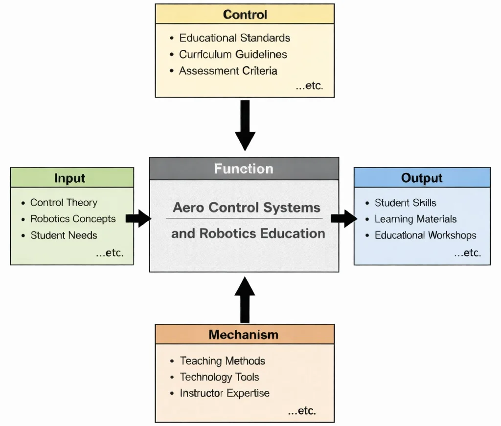
IDEF0 functional decomposition of Aero Control Systems and Robotics Education: control and robotics theory represent fundamental inputs structured by rigorous curriculum controls, executed via computational simulators and experimental mechanisms, and delivering verified engineering competencies alongside persistent open-access resources.

A futuristic aerospace control room with an operator watching multiple monitoring screens while satellites, an orbiting spacecraft, a rocket launch, and robotic astronauts appear above Earth in space.

Aero control systems and robotics operational paradigm: closing the real-time loop between high-bandwidth multi-spectral sensing, deterministic algorithmic decision-making, and microsecond actuator commands across atmospheric and deep-space operational domains.

This image portrays the heart of modern aero control and robotics: a human operator supervising complex systems through real-time dashboards and telemetry displays. In the foreground, layered screens suggest navigation, guidance, system health monitoring, and autonomous control loops. Above the Earth’s horizon, satellites and spacecraft represent communication links, positioning, and space operations, while the rocket launch hints at propulsion control and mission sequencing. Robotic figures in orbit evoke autonomous or remotely assisted robotics—machines designed to operate where humans face limits (vacuum, radiation, distance, and delay). The overall composition emphasizes closed-loop control: sensors collecting data, algorithms interpreting it, and actuators executing precise actions—whether stabilizing a vehicle, steering a spacecraft, or coordinating a robotic task.

Flight Dynamics and Mathematical Modeling

Unlike ground-based robots, aerospace systems move in three dimensions under continuous influence of gravity, lift, drag, and thrust. The dynamics of rigid-body flight are typically described using six degrees of freedom (6-DOF) referenced to body-fixed and Earth-centered inertial frames.

Translational motion follows Newton’s second law formulated in the rotating body frame:

$$\mathbf{F} = m \left( \frac{d\mathbf{v}}{dt} + \boldsymbol{\omega} \times \mathbf{v} \right)$$

Rotational motion is governed by Euler's rotational equations of motion:

$$\mathbf{I} \frac{d\boldsymbol{\omega}}{dt} + \boldsymbol{\omega} \times (\mathbf{I} \boldsymbol{\omega}) = \boldsymbol{\tau}$$

where:

$m$: Total mass of the aerospace vehicle ($\text{kg}$)
$\mathbf{v} = [u, v, w]^T$: Linear velocity vector in the body frame ($\text{m/s}$)
$\mathbf{I} \in \mathbb{R}^{3 \times 3}$: Vehicle mass moment of inertia tensor ($\text{kg}\cdot\text{m}^2$)
$\boldsymbol{\omega} = [p, q, r]^T$: Angular velocity rate vector containing roll, pitch, and yaw rates ($\text{rad/s}$)
$\boldsymbol{\tau} = [L, M, N]^T$: Resultant external moments and torques acting on the body ($\text{N}\cdot\text{m}$)
$\mathbf{F} = [X, Y, Z]^T$: Total aerodynamic, propulsive, and gravitational forces ($\text{N}$)

Accurate mathematical modeling is essential because even small parameter errors or unmodeled aerodynamic cross-couplings directly erode stability phase margins and controller robustness.

Worked Numerical Engineering Application: 6-DOF Cross-Coupling Pitch Dynamics

An autonomous high-speed atmospheric reconnaissance drone executes a high-rate rolling breakout maneuver. Calculate the total pitch angular acceleration $\dot{q} = \frac{dq}{dt}$ induced by inertial cross-coupling and aerodynamic elevator deflection under the following instantaneous state parameters:

Principal moments of inertia: $I_{xx} = 4.80 \text{ kg}\cdot\text{m}^2$, $I_{yy} = 12.50 \text{ kg}\cdot\text{m}^2$, $I_{zz} = 15.20 \text{ kg}\cdot\text{m}^2$ (with off-diagonal terms $I_{xy} = I_{yz} = I_{xz} \approx 0$)
Roll rate: $p = 4.20 \text{ rad/s}$
Yaw rate: $r = -1.80 \text{ rad/s}$
Applied net external pitching moment (aerodynamic elevator control authority): $M = -32.40 \text{ N}\cdot\text{m}$

Sequential Derivation & Calculation:

Step 1: Formulate Euler's pitch dynamic equation along the vehicle pitch axis (Y-body axis):

$$I_{yy} \dot{q} + (I_{xx} - I_{zz}) p r = M$$

Step 2: Algebraically isolate the angular acceleration $\dot{q}$:

$$\dot{q} = \frac{M - (I_{xx} - I_{zz}) p r}{I_{yy}}$$

Step 3: Evaluate the gyroscopic inertial cross-coupling torque term $\tau_{\text{inertial}} = (I_{xx} - I_{zz}) p r$:

$$\tau_{\text{inertial}} = (4.80 - 15.20) \times 4.20 \times (-1.80) = (-10.40) \times (-7.56) = +78.624 \text{ N}\cdot\text{m}$$

Step 4: Substitute the net moments into the isolated acceleration formulation:

$$\dot{q} = \frac{-32.40 - 78.624}{12.50} = \frac{-111.024}{12.50} = \mathbf{-8.88 \text{ rad/s}^2}$$

Analysis: Even though the commanded aerodynamic elevator moment is $-32.40 \text{ N}\cdot\text{m}$, the rolling-yawing cross-coupling produces an additional $-78.624 \text{ N}\cdot\text{m}$ inertial torque, precipitating a steep dynamic pitch-down acceleration of $\mathbf{-8.88 \text{ rad/s}^2}$. Modern multi-variable flight controllers must cancel these non-linear inertial cross-couplings in real time.

Stability and Control Surfaces

Aircraft stability depends on aerodynamic design, center of gravity placement, and control authority. Primary flight control surfaces—ailerons, elevators, and rudders—modify the camber and airflow over lifting surfaces to generate targeted restoring and maneuvering moments.

A fundamental longitudinal static stability criterion requires that the derivative of the pitching moment coefficient with respect to the angle of attack be strictly negative:

$$\frac{\partial C_m}{\partial \alpha} < 0$$

where:

$C_m$: Non-dimensional pitching moment coefficient about the aircraft center of gravity
$\alpha$: Angle of attack ($\text{rad}$ or $\text{deg}$)

A negative slope ensures that an uncommanded pitch-up gust ($\Delta \alpha > 0$) naturally induces a negative pitching moment ($\Delta C_m < 0$), driving the nose down to automatically re-establish trim equilibrium. Flight controllers operate within these aerodynamic boundaries, integrating principles developed in Advanced Control Systems in Robotics.

Guidance, Navigation, and Control (GNC)

Aerospace robotics is structured around the unified Guidance, Navigation, and Control (GNC) framework. These three subsystems execute continuously in closed feedback architectures to guarantee mission precision, dynamic stability, and flight envelope safety.

Guidance: Guidance determines the continuous optimal reference trajectory, path curvature vectors, or waypoint progression required to satisfy mission profiles. In autonomous UAVs, hypersonic vehicles, and spacecraft, guidance modules execute dynamic path replanning under terminal waypoint arrival criteria, obstacle envelopes, and energy budgets.
Navigation: Navigation estimates the true kinematic state vector—position $\mathbf{p}$, velocity $\mathbf{v}$, and attitude quaternion $\mathbf{q}$—by synthesizing multi-rate sensor inputs through recursive state estimators. Because satellite navigation signals face vulnerabilities, state estimators maintain observability through multi-sensor dead reckoning.
Control: Control computes and commands the precise physical forces and moments required to eliminate state tracking errors between the estimated navigation state and the guidance trajectory. Aerospace flight control loops regulate high-frequency inner loops (body rates) and outer loops (attitude and trajectory tracking) within certified stability margins.

Although GNC concepts appear in terrestrial robotics, aerospace implementations demand higher bandwidth, robust disturbance rejection against stochastic atmospheric turbulence, and formal deterministic safety verification under non-linear operational dynamics.

Autonomous UAV Systems

Unmanned Aerial Vehicles integrate tightly coupled embedded hardware and deterministic control software to sustain stable autonomous flight across dynamic operating regimes.

Flight Control Computer (FCC): The FCC executes deterministic real-time operating systems (RTOS) running stabilization loops at rates between $200 \text{ Hz}$ and $1000 \text{ Hz}$. It samples onboard avionics, executes state estimators, and computes control allocation algorithms without runtime jitter.
Electronic Speed Controllers (ESCs): ESCs regulate brushless DC (BLDC) motor rotor velocity by switching high-current field-effect transistors (FETs) via telemetry-driven digital protocols (such as DShot or CAN). Rapid motor response bandwidth is essential to multirotor differential torque attitude stabilization.
Inertial Measurement Units (IMUs): High-bandwidth tri-axial MEMS accelerometers and rate gyroscopes provide the fundamental kinematic rate measurements. Advanced avionics integrate multi-IMU arrays running real-time thermal compensation and bias tracking algorithms to prevent integration drift.
Radio Communication Links: Ground control links supply long-range telemetry feedback and supervisory mission tasking. Robust communication architectures incorporate frequency-hopping spread spectrum (FHSS) transceivers and secure data links capable of maintaining telemetry integrity across congested radio-frequency environments.
Redundant Power Systems: Multi-rail DC-DC power distribution units paired with isolated auxiliary battery backups isolate sensitive sensor avionics from motor back-EMF spikes and prevent brownouts during aggressive high-current maneuvering.

Together, these components constitute a real-time cyber-physical system in which high-speed computation, distributed sensing, and electro-mechanical actuation operate under strict aerodynamic boundaries.

Contemporary AI-Era Computational Paradigms in Aero Control

Modern aerospace control systems have expanded beyond purely classical single-input single-output loops, incorporating machine learning architectures and non-linear estimation frameworks directly into embedded flight computers:

1. Physics-Informed Neural Networks (PINNs) & Neural Operators: To resolve high-dimensional aerodynamic flow fields around complex airframes without running computationally prohibitive CFD in flight, surrogate neural models are trained directly on physics balance laws. Loss functions penalize deviations from Navier-Stokes equations:

$$\mathcal{L}_{\text{total}} = \mathcal{L}_{\text{data}} + \lambda_{\text{physics}} \|\mathcal{N}[\hat{u}] - f\|_{\Omega}^2$$

Fourier Neural Operators (FNOs) and DeepONets map continuous parameter spaces (such as changing Mach numbers, wing aeroelastic flexing, and control surface damage states) directly to full aerodynamic pressure fields in sub-millisecond execution times, enabling online real-time flight envelope protection.

Numerical Illustration: PINN Boundary Condition and Residual Loss Evaluation

Consider an online PINN surrogate predicting the spanwise circulation distribution $\Gamma(y)$ across an aeroelastic wing. At collocation point $y_k = 2.40 \text{ m}$, the empirical sensor-fused circulation observation is $\Gamma_{\text{meas}} = 14.80 \text{ m}^2/\text{s}$, while the network predicts $\hat{\Gamma} = 14.25 \text{ m}^2/\text{s}$. The physical Prandtl lifting-line governing residual evaluates to $\mathcal{R}_{\text{physics}} = \mathcal{N}[\hat{\Gamma}] - f = 0.35 \text{ m}^2/\text{s}$. Using a physics weight multiplier $\lambda_{\text{physics}} = 2.50$:

Step 1: Compute empirical supervised mean squared error component:

$$\mathcal{L}_{\text{data}} = (\hat{\Gamma} - \Gamma_{\text{meas}})^2 = (14.25 - 14.80)^2 = (-0.55)^2 = 0.3025$$

Step 2: Compute penalized physical residual component:

$$\lambda_{\text{physics}} \|\mathcal{R}_{\text{physics}}\|^2 = 2.50 \times (0.35)^2 = 2.50 \times 0.1225 = 0.30625$$

Step 3: Evaluate total composite loss driving the backpropagation gradient:

$$\mathcal{L}_{\text{total}} = 0.3025 + 0.30625 = \mathbf{0.6088}$$

2. Invariant Extended Kalman Filtering (IEKF) & Terrain-Relative Navigation (TRN): In GPS-denied, electronic-warfare, or planetary environments, classical EKF algorithms suffer from linearized covariance divergence because attitude and position errors are coupled across curved Lie group manifolds. Matrix Lie group state estimation ($SE_2(3)$) via Invariant EKFs ensures that state estimation error dynamics are strictly log-linear and state-trajectory independent.

Numerical Illustration: IEKF Lie Algebra Innovation and State Covariance Update

An autonomous vehicle navigating without GPS registers an optical terrain landmark located in global map coordinates at $\mathbf{p}_{\text{map}} = [120.00, 450.00, -80.00]^T \text{ m}$. The vehicle's predicted body-relative position is $\hat{\mathbf{p}} = [118.20, 451.10, -79.40]^T \text{ m}$.

Step 1: Calculate the 3D spatial innovation vector $\mathbf{z}$:

$$\mathbf{z} = \mathbf{p}_{\text{map}} - \hat{\mathbf{p}} = [120.00 - 118.20, 450.00 - 451.10, -80.00 - (-79.40)]^T = [1.80, -1.10, -0.60]^T \text{ m}$$

Step 2: With diagonal Kalman filter gain matrix $\mathbf{K} = \text{diag}(0.45, 0.45, 0.45)$, evaluate the state correction vector $\Delta \mathbf{x} = \mathbf{K} \mathbf{z}$:

$$\Delta \mathbf{x} = 0.45 \times [1.80, -1.10, -0.60]^T = [\mathbf{+0.81 \text{ m}}, \mathbf{-0.495 \text{ m}}, \mathbf{-0.27 \text{ m}}]^T$$

Step 3: Update updated body position $\hat{\mathbf{p}}^{+} = \hat{\mathbf{p}} + \Delta \mathbf{x}$:

$$\hat{\mathbf{p}}^{+} = [118.20 + 0.81, 451.10 - 0.495, -79.40 - 0.27]^T = \mathbf{[119.01, 450.605, -79.67]^T \text{ m}}$$

3. Edge Model Predictive Control (MPC): High-efficiency quadratic programming (QP) and active-set solvers execute directly on embedded flight microprocessors. Embedded non-linear MPC iteratively optimizes vehicle trajectories over a finite receding horizon:

$$\min_{\mathbf{u}} \int_{t}^{t+T} \left( \|\mathbf{x}(\tau) - \mathbf{x}_{\text{ref}}(\tau)\|_{\mathbf{Q}}^2 + \|\mathbf{u}(\tau)\|_{\mathbf{R}}^2 \right) d\tau \quad \text{subject to} \quad \dot{\mathbf{x}} = f(\mathbf{x}, \mathbf{u}), \quad \mathbf{u}_{\min} \le \mathbf{u} \le \mathbf{u}_{\max}$$

Numerical Illustration: Discrete-Time Receding Horizon Stage Cost Calculation

Consider a single discrete MPC prediction stage where state deviation is pitch angle error $e_\theta = 0.08 \text{ rad}$ and control actuation is elevator deflection $\delta_e = 0.12 \text{ rad}$. The performance weighting matrices are scalar values $Q = 500 \text{ N}\cdot\text{m/rad}^2$ and $R = 120 \text{ N}\cdot\text{m/rad}^2$.

Step 1: Calculate state trajectory penalty:

$$J_{\text{state}} = Q \cdot e_\theta^2 = 500 \times (0.08)^2 = 500 \times 0.0064 = 3.20$$

Step 2: Calculate actuator effort expenditure penalty:

$$J_{\text{control}} = R \cdot \delta_e^2 = 120 \times (0.12)^2 = 120 \times 0.0144 = 1.728$$

Step 3: Total instantaneous stage optimization cost:

$$J_{\text{stage}} = J_{\text{state}} + J_{\text{control}} = 3.20 + 1.728 = \mathbf{4.928}$$

Telemetry and Communication Constraints

Aerospace systems rely on telemetry for monitoring, diagnostics, and mission coordination.

Unlike industrial robots connected through wired networks, aerial platforms depend on wireless communication channels that may experience latency, interference, or signal loss. Designers must therefore ensure that core stabilization remains fully autonomous. Communication systems support supervision and data logging, but flight safety cannot depend exclusively on external control.

Redundancy and Safety Engineering

Reliability in aerospace robotics is not optional—it is fundamental to safe operation.

Dual or Triple Sensor Architectures: Multiple IMUs or GPS modules allow cross-verification of measurements. If one sensor produces anomalous data, fault-detection algorithms isolate it without destabilizing the system.
Redundant Processors: Backup control processors can assume command if the primary unit fails. This reduces single-point failure risk in safety-critical missions.
Fail-Safe Modes: Automatic return-to-home procedures, controlled descent algorithms, or thrust reduction strategies activate when abnormal conditions are detected. These safeguards protect both the vehicle and its surroundings.

Such redundancy increases weight and cost, yet aerospace engineering prioritizes safety margins over minimal hardware.

Applications in Space Robotics

Beyond atmospheric flight, robotics extends into orbital, lunar, and interplanetary regimes where environmental boundary conditions diverge radically from Earth flight dynamics: the absence of aerodynamic damping, intense thermal cycling ($\pm 150^\circ\text{C}$), hard radiation, and vacuum conditions eliminate conventional aerodynamics and introduce non-linear multi-body dynamics.

1. Orbital Rendezvous, Proximity Operations, and Docking (RPOD): Autonomous spacecraft rendezvous is governed by relative orbital mechanics rather than terrestrial kinematics. For two spacecraft in circular Low Earth Orbit (LEO), relative translational motion between the robotic chaser and target is formulated using the linear Clohessy-Wiltshire (Hill's) equations:

$$\ddot{x} - 2n\dot{y} - 3n^2 x = \frac{F_x}{m}, \quad \ddot{y} + 2n\dot{x} = \frac{F_y}{m}, \quad \ddot{z} + n^2 z = \frac{F_z}{m}$$

where $x$ represents radial displacement from Earth, $y$ is along-track along the target velocity vector, $z$ is out-of-plane cross-track, $n = \sqrt{\mu / r_0^3}$ is orbital mean motion, and $[F_x, F_y, F_z]^T$ are cold-gas or hypergolic thruster firing forces. In terminal docking, LiDAR-based point cloud registration algorithms (such as Iterative Closest Point, ICP) run onboard to guide capture mechanisms into millimeter-level alignment.

Worked Numerical Example: Clohessy-Wiltshire Orbital Cross-Track Restoring Force

A servicing satellite of mass $m = 450 \text{ kg}$ operates in a circular orbit at altitude $h = 400 \text{ km}$ ($r_0 = 6778 \text{ km}$, standard gravitational parameter $\mu = 3.986 \times 10^{14} \text{ m}^3/\text{s}^2$). Calculate the out-of-plane cross-track gravitational acceleration and required thruster holding force when the chaser holds a static out-of-plane offset of $z = 25.0 \text{ m}$.

Step 1: Calculate the orbital mean motion $n$:

$$n = \sqrt{\frac{\mu}{r_0^3}} = \sqrt{\frac{3.986 \times 10^{14} \text{ m}^3/\text{s}^2}{(6.778 \times 10^6 \text{ m})^3}} = \sqrt{\frac{3.986 \times 10^{14}}{3.114 \times 10^{20}}} = \sqrt{1.280 \times 10^{-6}} = 1.131 \times 10^{-3} \text{ rad/s}$$

Step 2: Evaluate the out-of-plane natural orbital restoring acceleration ($\ddot{z}_{\text{orbit}} = -n^2 z$):

$$\ddot{z}_{\text{orbit}} = -(1.131 \times 10^{-3} \text{ rad/s})^2 \times 25.0 \text{ m} = -(1.280 \times 10^{-6}) \times 25.0 = -3.20 \times 10^{-5} \text{ m/s}^2$$

Step 3: Calculate required continuous thruster opposing force $F_z = m \cdot |\ddot{z}_{\text{orbit}}|$ to maintain station-keeping:

$$F_z = 450 \text{ kg} \times 3.20 \times 10^{-5} \text{ m/s}^2 = \mathbf{0.0144 \text{ N} \quad (14.4 \text{ mN})}$$

Analysis: Without active propulsion of $14.4 \text{ mN}$, the robotic servicer will oscillate harmonically across the target's orbital plane with a period equal to the orbit ($T = 2\pi/n \approx 5555 \text{ s} \approx 92.6 \text{ minutes}$).

2. Free-Floating Space Manipulators and Non-Holonomic Coupling: Satellite servicing arms (such as the Canadarm2 on the ISS or robotic active debris removal claws) operate under free-floating dynamics. Because the spacecraft base is not anchored to a massive ground plane, moving a manipulator joint induces equal and opposite angular momentum reactions in the base satellite:

$$\mathbf{I}_{\text{base}} \dot{\boldsymbol{\omega}}_{\text{base}} + \mathbf{J}_{\text{arm}}^T \boldsymbol{\tau}_{\text{joints}} = \mathbf{0}$$

To position the end-effector accurately without expending limited satellite attitude thruster fuel, control engineers use the Generalized Jacobian Matrix ($\mathbf{J}^*$). This mathematical operator maps desired end-effector cartesian velocities $\dot{\mathbf{x}}_e$ directly to joint rate commands $\dot{\mathbf{q}}$ while simultaneously accounting for the free dynamic recoil of the satellite bus:

$$\dot{\mathbf{x}}_e = \mathbf{J}^*(\mathbf{q}) \dot{\mathbf{q}}$$

3. Autonomous Planetary Exploration Rovers: Planetary robotics (such as the Mars Perseverance or lunar VIPER rovers) must navigate extreme terrain under one-way signal propagation latencies ranging from 4 to 22 minutes. At these communication delays, closed-loop driving from Earth is impossible. Autonomous rovers utilize real-time Stereo Visual Odometry (VO) fused with wheel odometry slip-detection to estimate slip in loose regolith. When wheel slippage exceeds 40%, autonomous path planners replan local traversals to prevent rover immobilization.

Engineering Trade-offs

Designing aerospace control systems and robotic architectures requires balancing conflicting physical, computational, and regulatory constraints. In safety-critical aerospace missions, performance improvements in one dimension inevitably impose severe penalties across mass, power, or operational margins:

Design Trade-off	Primary Benefit	Systemic Penalty / Risk	Quantitative Design Metric
Static Stability vs. Maneuverability	Inherent aerodynamic restoring moment; vehicle recovers naturally from wind gusts without computer intervention.	High trim drag; reduced pitch agility; requires larger control surfaces and actuator force to execute sharp turns.	Static Margin ($\text{SM} = \frac{x_{\text{np}} - x_{\text{cg}}}{\bar{c}}$). Commercial aircraft: $+5\%$ to $+10\%$; Fighter aircraft: $-2\%$ to $-5\%$.
High Gain ($K_p, K_d$) vs. Actuator Saturation	Ultra-fast disturbance rejection; tight trajectory tracking; minimized steady-state error.	Actuator rate and deflection limits reached; high-frequency servo chattering; severe motor overheating and gear wear.	Actuator Bandwidth ($\omega_{\text{act}} \ge 3 \times \omega_{\text{bandwidth}}$); Phase Margin ($\ge 45^\circ$); Gain Margin ($\ge 6 \text{ dB}$).
Sensor Redundancy vs. SWaP-C	Eliminates single points of failure via Triple Modular Redundancy (TMR); enables real-time fault detection and isolation.	Significantly increases mass, electrical power draw, thermal dissipation, avionics bay volume, and procurement cost.	Mean Time Between Failures ($\text{MTBF} > 10^9 \text{ flight hours}$ for certified civil transport flight controls).
Model Complexity vs. Real-Time Execution	Predicts complex unsteady aerodynamic couplings, aeroelastic flexibility, and localized stall effects.	High compute latency; exceeding real-time loop deadlines introduces unmodeled phase lag, destabilizing high-speed control loops.	Loop Execution Margin: Algorithm execution time $\tau_{\text{exec}} \le 0.4 \times \Delta t_{\text{loop}}$ (e.g., $< 0.8 \text{ ms}$ for a $500 \text{ Hz}$ loop).

Quantitative Trade-off Illustration: Static Margin vs. Control Power Budget

Consider an aerial vehicle of weight $W = 20,000 \text{ N}$ with mean aerodynamic chord $\bar{c} = 2.0 \text{ m}$. If the vehicle is configured with a strongly stable Static Margin of $\text{SM} = +0.12$ (12%), the center of gravity ($x_{\text{cg}}$) sits $0.24 \text{ m}$ ahead of the aerodynamic neutral point ($x_{\text{np}}$). To pitch the nose up by generating an angle of attack increment that produces $\Delta L = 4,000 \text{ N}$ of lift, calculate the opposing aerodynamic pitch-down moment $M_{\text{restoring}}$ that the elevator actuator must overcome:

Step 1: Calculate the moment arm $d = \text{SM} \cdot \bar{c}$:

$$d = 0.12 \times 2.0 \text{ m} = 0.24 \text{ m}$$

Step 2: Calculate the restoring moment:

$$M_{\text{restoring}} = \Delta L \times d = 4,000 \text{ N} \times 0.24 \text{ m} = \mathbf{960.0 \text{ N}\cdot\text{m}}$$

Comparison: If designed with relaxed static stability ($\text{SM} = -0.02$), the elevator requires zero trim moment to initiate pitch-up and only needs to arrest the divergence, reducing the required elevator surface area by 40% and saving structural weight, but making digital flight computer stabilization strictly mandatory.

Preparation for University-Level Study

Students interested in aero control systems and robotics should build strong foundations in:

Flight Dynamics and Aerodynamics: Understanding lift, drag, moment coefficients, and stability derivatives is essential for modeling aerial systems.
Control Systems and Stability Analysis: Feedback control theory, state-space modeling, and stability margins form the mathematical basis of flight regulation.
Embedded Avionics Systems: Real-time processors, sensor integration, and fault detection mechanisms are central to autonomous aerospace platforms.
Sensor Fusion and Navigation: Kalman filtering, inertial navigation, and GPS integration are crucial for robust state estimation.

Aerospace robotics reveals how intelligence must coexist with physics at high speed and high consequence. It is where mathematics meets airflow, and where stability is not optional but essential.

Aerospace & Aeronautical Engineering Hub

Acts as the central curriculum node, connecting flight dynamics, propulsion, structural mechanics, and avionics into a unified systems-engineering roadmap.

Aero Control Systems & Robotics

Explores dynamic modeling, feedback stability loops, sensor fusion (IMU/GPS), autonomous GNC architectures, and fault-tolerant robotic flight controllers.

Avionics

Focuses on real-time flight management computers, glass cockpit interfaces, radar, communication links, and safety-critical embedded systems hardware.

Flight Mechanics

Details 6-DOF vehicle equations of motion, trim states, static/dynamic stability derivatives, and maneuvering envelope constraints essential for control law design.

Spacecraft Engineering

Examines orbital guidance, reaction wheel attitude control, thruster actuation, and autonomous docking mechanisms operating in microgravity environments.

Robotics & Automation in EE

Covers power electronics, motor drives, signal conditioning hardware, microcontrollers, and sensor interfaces enabling physical actuation.

Robotics & Automation in Mech Eng

Focuses on structural linkage kinematics, joint torque transmission, gearboxes, end-effector mechanics, and heavy payload handling.

Interactive Flight Attitude PID Closed-Loop Controller Simulator

Adjust Proportional ($K_{\text{p}}$), Integral ($K_{\text{i}}$), and Derivative ($K_{\text{d}}$) gains to observe how a closed-loop flight attitude controller restores stability when exposed to sudden turbulent wind gusts.

Proportional Gain ($K_{\text{p}}$): 2.5

Integral Gain ($K_{\text{i}}$): 0.2

Derivative Gain ($K_{\text{d}}$): 1.2

Current Pitch Angle ($\theta$): 0.00°

Attitude Error ($e$): 0.00°

Control Output ($\delta_{\text{e}}$): 0.00

Interactive runtime environment: https://prep4uni.online/stem/physical-technologies/aerospace-and-aeronautical-engineering/aero-control-systems-and-robotics/

Interactive Concept Review

Why must guidance, navigation, and control (GNC) operate as tightly coupled loops in autonomous UAVs?

Guidance provides the reference path targets, Navigation computes the vehicle’s dynamic kinematic state via sensor fusion, and Control generates instantaneous actuator commands to eliminate tracking errors. If any link experiences excessive latency, sensor bias, or state divergence, the control loop can inject incorrect forces, rapidly leading to dynamic instability, structural overstress, or catastrophic flight boundary violations.

What is the mathematical condition for static pitch stability in longitudinal flight dynamics?

Static pitch stability requires that the partial derivative of the pitching moment coefficient with respect to angle of attack ($\partial C_m / \partial \alpha$) be strictly negative ($< 0$). This ensures that an upward pitch disturbance ($\Delta \alpha > 0$) generates an opposing nose-down aerodynamic moment ($\Delta C_m < 0$) that automatically restores flight equilibrium without requiring active control intervention.

How do space robotic manipulators handle dynamic coupling in microgravity environments?

Without a fixed gravitational anchor or mechanical foundation, articulating a robotic arm in microgravity induces equal and opposite reaction forces and torques onto the host spacecraft bus (governed by the conservation of total angular and linear momentum). Control algorithms must compensate for this reaction motion using reaction wheel counter-torquing, momentum management desaturation, or generalized Jacobian trajectory optimization to maintain precise pointing of high-gain communication antennas and solar arrays.

Frequently Asked Questions

How is robotics different in aerospace engineering compared to industrial robotics?

Aerospace robotics operates under strict aerodynamic, stability, and safety constraints. Unlike factory robots, aerial and space systems must maintain dynamic equilibrium in three-dimensional environments where gravity, airflow, and inertia continuously interact. Flight stability margins and guidance precision are critical.

Why is stability analysis so important in aero control systems?

Aircraft and UAVs must remain stable under disturbances such as turbulence, wind gusts, and payload changes. Stability analysis ensures that small deviations in attitude or velocity do not grow uncontrollably. Control laws are designed with safety margins to maintain predictable flight behavior.

What role do sensors play in aerospace robotics?

Aerospace systems rely heavily on inertial measurement units (IMUs), GPS receivers, airspeed sensors, pressure sensors, and radar or vision systems. These sensors provide state information necessary for attitude estimation, navigation, and autonomous guidance.

How are control surfaces and actuators integrated in UAV systems?

Actuators drive control surfaces such as ailerons, elevators, and rudders. Electrical and servo systems must respond quickly and accurately to maintain stability. Actuator bandwidth and reliability directly affect flight performance.

What is guidance, navigation, and control (GNC)?

Guidance determines the desired trajectory, navigation estimates the vehicle’s current state, and control generates actuator commands to follow the trajectory. Together, GNC systems enable autonomous flight, precision landing, and mission execution.

Why is redundancy critical in aerospace robotics?

Aerospace systems often incorporate redundant sensors, processors, and communication links to ensure reliability. Failure tolerance is essential because system malfunction can have severe safety consequences.

How does telemetry support aerospace robotic operations?

Telemetry systems transmit flight data to ground stations for monitoring and analysis. Real-time data links enable supervision, diagnostics, and mission adjustments, particularly in long-range UAV or spacecraft operations.

End-of-Page Comprehensive Practice Module

Foundational Concept Review

What are the three core elements comprising the GNC architecture in aerospace engineering? Answer: The three core elements are Guidance (determining target path/waypoints), Navigation (estimating current vehicle state via sensor fusion), and Control (generating actuator commands to track guidance trajectory).
Define six degrees of freedom (6-DOF) as applied to an unconstrained aerospace body in space. Answer: 6-DOF represents three translational motions along perpendicular axes (surge/X, sway/Y, heave/Z) and three rotational motions about those axes (roll/$\phi$, pitch/$\theta$, yaw/$\psi$).
What primary physical measurements are collected by an Inertial Measurement Unit (IMU)? Answer: An IMU measures linear acceleration using accelerometers and angular velocity rates using gyroscopes across three orthogonal axes.
Explain why Electronic Speed Controllers (ESCs) are crucial in multirotor UAV flight control. Answer: Multirotor UAVs rely on differential motor thrust for attitude control; ESCs quickly adjust high-frequency pulse-width modulation (PWM) power signals to brushless motors based on flight computer commands.
What is anti-windup clamping in an integral control loop? Answer: Anti-windup clamping limits the accumulation of error in the integral term when actuators saturate, preventing extreme overshoot or delayed recovery once errors reverse direction.
Distinguish between open-loop and closed-loop control in aircraft systems. Answer: Open-loop control executes preset actuator inputs without measuring actual system response, while closed-loop control uses sensor feedback to continuously measure attitude/velocity error and apply corrective forces.
Define a fail-safe flight mode in autonomous aerial robotics. Answer: A fail-safe mode is a pre-programmed emergency algorithm (e.g., Return-To-Home, automated parachuting, hover-and-land) that triggers automatically when critical events like signal loss or battery depletion occur.
What role do reaction wheels play in satellite attitude control? Answer: Reaction wheels spin electric flywheels to store angular momentum, allowing precise satellite orientation adjustments in vacuum via conservation of angular momentum without expending propellant.

Analytical & Systems Engineering Challenges

Analyze the trade-offs involved in selecting between sensor-driven fully autonomous UAV control and human-in-the-loop supervisory telemetry control. Answer: Fully autonomous control provides ultra-fast microsecond stabilization loop bandwidth and operates reliably during communication blackouts, but lacks human contextual adaptability in unstructured edge-case environments. Telemetry supervision introduces human decision-making, but suffers from wireless link latency, signal dropouts, and bandwidth constraints.
Evaluate why Sensor Fusion using Kalman Filtering is necessary when combining GPS data with IMU telemetry for UAV navigation. Answer: IMUs provide high-frequency ($100\text{--}1000 \text{ Hz}$) motion tracking but accumulate unbounded integration drift over time. GPS provides absolute spatial positioning without drift, but updates at low rates ($1\text{--}10 \text{ Hz}$) and is prone to signal dropouts. An Extended Kalman Filter dynamically fuses both signals to yield a smooth, drift-free, high-rate state estimate.
Explain how dynamic coupling between manipulator arm joints complicates attitude control on an orbiting spacecraft servicing platform. Answer: When a robotic arm rotates in microgravity, equal and opposite reaction torques propagate into the spacecraft chassis. Without active attitude compensation from reaction wheels or thrusters, the entire satellite will counter-rotate, disturbing solar panel alignment and directional communications antennas.
Discuss the system-level consequences of controller gain selection ($K_{\text{p}}$, $K_{\text{i}}$, $K_{\text{d}}$) on control surface servo motor heating and mechanical fatigue. Answer: Overly aggressive gains (especially high derivative gain $K_{\text{d}}$) cause the flight controller to amplify sensor noise, resulting in high-frequency control surface "chatter." This excessive actuator activity leads to severe overheating in servo electronics, rapid mechanical gear wear, and high battery power drain.
Why do safety-critical avionics computers utilize triple-modular redundancy (TMR) with voting logic? Answer: TMR runs three independent processors executing identical control algorithms simultaneously. A hardware voting circuit compares outputs; if a single processor suffers a memory corruption or hardware fault, the voter selects the matching outputs of the remaining two, enabling uninterrupted flight safety without single-point failure.
Contrast the control authority requirements of fixed-wing aircraft control surfaces with multirotor thrust-vectoring in turbulent atmospheric conditions. Answer: Fixed-wing control surface authority depends directly on dynamic pressure ($q = \frac{1}{2} \rho V^2$); at low airspeeds, elevator/aileron effectiveness drops significantly. Multirotor thrust-vectoring alters rotor motor RPMs directly, maintaining high control torque independent of forward airspeed, though vulnerable to high wind gust drag.
Describe how sensor latency in an attitude estimation loop alters control loop phase margin and system stability. Answer: Sensor filter delay introduces time lags into feedback signals. In frequency domain terms, time delay adds linear phase lag ($-\omega T$) proportional to frequency, eroding system phase margin and potentially converting negative feedback into positive feedback, inducing unstable hunting oscillations.

Quantitative Calculations & Applied Analysis

A $3.0 \text{ kg}$ drone experiences an uncompensated lateral aerodynamic wind force of $12.0 \text{ N}$. Calculate the resulting translational linear acceleration. Answer:
Step 1: Apply Newton's Second Law: $F = m \cdot a \Rightarrow a = \frac{F}{m}$
Step 2: Substitute values: $a = \frac{12.0 \text{ N}}{3.0 \text{ kg}} = \mathbf{4.0 \text{ m/s}^2}$
An altitude pitch loop exhibits an attitude error $e = -0.15 \text{ rad}$ ($-8.59^\circ$). Given a proportional controller gain $K_{\text{p}} = 4.0$, calculate the proportional control torque output. Answer:
Step 1: Apply the proportional control law: $u_{\text{P}} = K_{\text{p}} \cdot e$
Step 2: Substitute values: $u_{\text{P}} = 4.0 \times (-0.15 \text{ rad}) = \mathbf{-0.60 \text{ N}\cdot\text{m}}$
Calculate the moment of inertia ($I$) required for a spacecraft reaction wheel if an angular acceleration $\alpha = 2.5 \text{ rad/s}^2$ must be generated using an electric motor torque $\tau = 0.50 \text{ N}\cdot\text{m}$. Answer:
Step 1: Rotational formula: $\tau = I \cdot \alpha \Rightarrow I = \frac{\tau}{\alpha}$
Step 2: Substitute values: $I = \frac{0.50 \text{ N}\cdot\text{m}}{2.5 \text{ rad/s}^2} = \mathbf{0.20 \text{ kg}\cdot\text{m}^2}$
An aircraft pitched up has a pitching moment coefficient derivative $\frac{\partial C_m}{\partial \alpha} = -0.8 \text{ rad}^{-1}$. If angle of attack increases by $\Delta \alpha = +0.05 \text{ rad}$, calculate the change in pitching moment coefficient ($\Delta C_m$). Answer:
Step 1: Formula: $\Delta C_m = \left( \frac{\partial C_m}{\partial \alpha} \right) \times \Delta \alpha$
Step 2: Substitute values: $\Delta C_m = -0.8 \times 0.05 = \mathbf{-0.04}$ (Restoring nose-down moment generated)
A quadrotor flight controller samples IMU gyro data at $500 \text{ Hz}$. Determine the loop time step ($\Delta t$) in milliseconds between consecutive sensor readings. Answer:
Step 1: Time step formula: $\Delta t = \frac{1}{f}$
Step 2: $\Delta t = \frac{1}{500 \text{ s}^{-1}} = 0.002 \text{ s} = \mathbf{2.0 \text{ ms}}$
Calculate the derivative term output ($u_{\text{D}}$) for a flight pitch controller with gain $K_{\text{d}} = 1.5$, given a current pitch error $e_k = 0.04 \text{ rad}$, previous error $e_{k-1} = 0.01 \text{ rad}$, and time step $\Delta t = 0.01 \text{ s}$. Answer:
Step 1: Calculate the error rate of change: $\frac{de}{dt} = \frac{e_k - e_{k-1}}{\Delta t} = \frac{0.04 - 0.01}{0.01} = \frac{0.03}{0.01} = 3.0 \text{ rad/s}$
Step 2: Calculate derivative output: $u_{\text{D}} = K_{\text{d}} \times \left( \frac{de}{dt} \right) = 1.5 \times 3.0 = \mathbf{4.50}$
A satellite with moment of inertia $I = 1200 \text{ kg}\cdot\text{m}^2$ experiences a constant cold-gas thruster torque $\tau = 6.0 \text{ N}\cdot\text{m}$ for $4.0 \text{ seconds}$. Calculate the resulting change in angular velocity ($\Delta \omega$). Answer:
Step 1: Calculate angular acceleration: $\alpha = \frac{\tau}{I} = \frac{6.0 \text{ N}\cdot\text{m}}{1200 \text{ kg}\cdot\text{m}^2} = 0.005 \text{ rad/s}^2$
Step 2: Calculate angular velocity change: $\Delta \omega = \alpha \times t = 0.005 \text{ rad/s}^2 \times 4.0 \text{ s} = \mathbf{0.02 \text{ rad/s}}$

← Back to Aerospace & Aeronautical Engineering Hub

Last updated: 23 Sep 2026