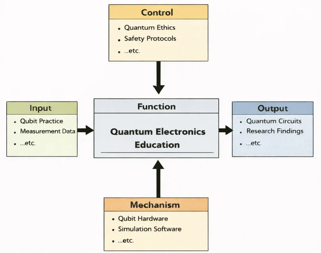
Prepare for University Studies & Career Advancement

Quantum Electronics

Quantum Electronics Education represents the frontier where solid-state physics, electrodynamics, and quantum mechanics converge to manipulate matter and light at the single-quanta limit. The discipline begins with fundamental physical Inputs—coherent laser photons, microwave control pulses, Josephson junction tunneling states, and cryogenic sensor signals. These inputs are governed by rigorous Controls, including quantum non-demolition measurement protocols, decoherence limits, and cryogenic safety standards. Supported by sophisticated Mechanisms such as dilution refrigerators, traveling-wave parametric amplifiers (TWPAs), and microwave arbitrary waveform generators (AWGs), students transform quantum phenomena into practical engineering outcomes. The resulting Outputs include scalable superconducting qubit circuits, quantum key distribution (QKD) transceivers, and ultra-sensitive quantum metrology instruments that form the foundation of next-generation computation and secure communications.

Figure 1: IDEF0 architectural view of Quantum Electronics Education: transforming microscopic quantum states into validated solid-state devices and quantum information hardware.

Quantum Electronics is an advanced frontier within Electrical and Electronic Engineering, bridging microscopic quantum mechanics with physical electronic systems. By manipulating discrete quantum states—such as electron spin, photon polarization, and superconducting Cooper pairs—quantum engineers design devices that surpass classical physical ceilings in computational throughput, measurement sensitivity, and communications security.

The foundations of quantum device fabrication and high-frequency microwave transmission depend heavily on principles from Electronics Engineering and nanometer-scale lithography studied in Embedded Systems and Microelectronics. High-speed microwave control lines require precision signal conditioning and filtering derived from Signal Processing to mitigate phase noise and preserve fragile superposition states.

To measure delicate quantum signals without inducing wave-function collapse, quantum systems integrate low-noise cryogenic amplifiers and metrological calibration techniques from Instrumentation and Measurement. In quantum communication networks and Quantum Key Distribution (QKD), quantum electronics interfaces directly with optical transceivers and photon routing protocols developed in Communication Engineering.

Furthermore, active stabilization of qubit states against environmental dephasing relies on closed-loop feedback and optimal control theory established in Control Systems Engineering. As quantum sensing technologies mature, they enable revolutionary applications in Biomedical Electronics through ultra-sensitive magnetoencephalography (MEG) using optically pumped magnetometers, while distributed quantum sensors expand the frontiers of the Internet of Things (IoT) and Smart Technologies.

In power infrastructure, quantum electronics underpins the study of high-temperature superconducting cables that eliminate transmission losses in Power Systems Engineering, and advances quantum-dot photovoltaic cells explored in Renewable Energy and Energy Storage. Simultaneously, robotic manipulators in Robotics and Automation in E&E benefit from quantum inertial navigation units operating without GPS dependency.

Beyond electrical hardware, quantum instrumentation informs environmental research in Environmental Engineering, supporting trace gas spectroscopy in Air Quality Engineering and isotope sensing in Environmental Monitoring and Data Analysis. Students pursuing Quantum Electronics acquire rigorous mathematical, physical, and computational competencies, positioning themselves at the cutting edge of modern science and industry.

Interactive Two-Level Qubit Dynamics: Rabi Oscillations & Decoherence

Simulate the quantum state evolution of a driven superconducting transmon qubit. Adjust the Rabi drive amplitude ($\Omega_R$), frequency detuning ($\Delta$), and transverse dephasing time ($T_2^*$) to observe coherent state transitions between $|0\rangle$ and $|1\rangle$.

Rabi Frequency $\Omega_R$ (MHz): 20

Detuning $\Delta$ (MHz): 0.0

Dephasing Time $T_2^*$ ($\mu\text{s}$): 0.25

Effective Rabi Frequency ($\Omega_{\text{eff}}$): 20.00 MHz

Excited State Pop. $P_{|1\rangle}$: 0.00

$\pi$-Pulse Duration ($t_\pi$): 25.0 ns

Simulation runtime engine: Prep4Uni.Online Quantum Electronics Hub

Physicist inspecting a golden dilution refrigerator stage with glowing quantum processors, microwave waveguides, and holographic qubit state readouts

Figure 2: Quantum Electronics — engineering solid-state quantum chips, cryogenic microwave control interfaces, and coherent quantum state systems.

The illustration shows a quantum computing cleanroom where an engineer inspects the lowest stage of a dilution refrigerator. Gilded thermal plates, coaxial semi-rigid microwave cables, and magnetic shielding house a superconducting quantum processor operating at millikelvin temperatures. Holographic readouts display Bloch sphere rotations, energy level spacings, and quantum error syndrome measurements—capturing how quantum electronics translates atomic-scale quantum mechanics into physical, controllable solid-state architectures.

Quantum Electronics: Curriculum Roadmap & Cluster Navigation

Electrical & Electronic Engineering Overview

Provides the macro-disciplinary foundation linking classical electromagnetic theory with quantum information devices.

Quantum Electronics (Current Page)

Engineers solid-state devices operating at single-quanta limits, spanning qubits, Josephson junctions, and quantum photonics.

Electronics Engineering

Designs the cryogenic semiconductor amplifiers, low-noise mixers, and microwave filters controlling quantum hardware.

Embedded Systems & Microelectronics

Implements real-time FPGA and cryogenic CMOS controllers to execute nanosecond-scale quantum control sequences.

Instrumentation & Measurement

Executes quantum non-demolition measurements, heterodyne dispersive readout, and ultra-low-noise calibration.

Communication Engineering

Deploys Quantum Key Distribution (QKD), single-photon detectors, and quantum repeaters for unhackable networks.

Control Systems Engineering

Applies quantum optimal control (GRAPE, DRAG) to suppress leakage errors and steer coherent state trajectories.

Signal Processing

Demodulates weak dispersive readout tones, applying matched filtering and machine learning state discrimination.

IoT & Smart Technologies

Integrates quantum diamond NV-center sensors into distributed edge networks for extreme physical metrology.

Power Systems & Energy Storage

Applies superconducting magnetic energy storage (SMES) and quantum dots to optimize utility-scale energy conversion.

Biomedical Electronics

Deploys optically pumped magnetometers (OPMs) for non-invasive, room-temperature functional brain imaging.

Robotics & Automation in EE

Employs cold-atom quantum gravimeters and gyroscopes for high-precision GPS-denied autonomous navigation.

Core Concepts in Quantum Electronics

Quantum electronics operates where the discrete nature of energy levels, quantum phase coherence, and macroscopic wave functions dictate circuit behavior. Unlike classical circuits described by Kirchhoff's laws and Ohm's law, quantum electronic circuits treat charge and magnetic flux as non-commuting quantum operators:

Macroscopic Quantum Tunneling and Josephson JunctionsWhen two superconducting electrodes are separated by an ultra-thin insulating barrier ($\sim 1\text{--}2\,\text{nm}$), Cooper pairs tunnel coherently across the junction without voltage drop. Governed by the DC and AC Josephson relations: $$I(t) = I_c \sin(\phi(t)), \qquad \frac{d\phi(t)}{dt} = \frac{2e}{\hbar} V(t)$$ where $I_c$ is the critical current and $\phi$ is the gauge-invariant superconducting phase difference. Because the junction acts as a non-dissipative, non-linear inductor $L_J(\phi) = \frac{\Phi_0}{2\pi I_c \cos(\phi)}$, it introduces anharmonicity into superconducting LC resonators, separating the $|0\rangle \to |1\rangle$ transition from higher energy levels to form addressable qubits.
Circuit Quantum Electrodynamics (cQED)Circuit QED adapts cavity quantum electrodynamics to solid-state chips by coupling a superconducting artificial atom (transmon qubit) to a superconducting coplanar waveguide resonator. In the dispersive regime where qubit-resonator detuning $|\Delta| = |\omega_q - \omega_r| \gg g$ (where $g$ is the vacuum Rabi coupling strength), the interaction Hamiltonian is: $$\hat{H}_{\text{disp}} \approx \hbar (\omega_r + \chi \hat{\sigma}_z) \hat{a}^\dagger \hat{a} + \frac{1}{2} \hbar \omega_q \hat{\sigma}_z$$ The cavity resonance frequency shifts by $\pm \chi$ depending on whether the qubit occupies the ground state $|0\rangle$ or excited state $|1\rangle$, enabling fast quantum non-demolition (QND) dispersive readout using microwave probe tones.
Coherence Times, Decoherence, and DephasingA physical qubit's operational fidelity is constrained by two fundamental relaxation processes:
- Energy Relaxation Time ($T_1$): The characteristic timescale over which an excited state $|1\rangle$ decays spontaneously to $|0\rangle$ by emitting energy into dielectric loss channels, quasiparticles, or radiative modes.
- Transverse Dephasing Time ($T_2^*$): The timescale over which phase coherence between superposition components $\frac{1}{\sqrt{2}}(|0\rangle + |1\rangle)$ is lost due to low-frequency $1/f$ magnetic flux noise, charge fluctuations, and photon shot noise, governed by $\frac{1}{T_2} = \frac{1}{2 T_1} + \frac{1}{T_\phi}$.
Cryogenic Microwave Control & Attenuation ChainsSuperconducting qubits operate at frequencies around $4\text{--}8\,\text{GHz}$, corresponding to an energy transition $h \nu \approx 20\text{--}30\,\mu\text{eV}$. To prevent room-temperature blackbody thermal photons ($k_B T \gg h\nu$ at $300\,\text{K}$) from swamping the qubit, control lines inside dilution refrigerators incorporate distributed cryogenic attenuators ($20\,\text{dB}$ at $4\,\text{K}$, $20\,\text{dB}$ at $100\,\text{mK}$, $20\,\text{dB}$ at the $10\,\text{mK}$ mixing chamber plate) to thermalize incoming microwave coax lines down to sub-photon noise floors.
Solid-State Quantum Defect CentersBeyond superconducting circuits, quantum electronics manipulates localized atomic defects in semiconductors, such as Nitrogen-Vacancy (NV) centers in diamond and divacancies in Silicon Carbide (SiC). These defects exhibit optically addressable electron spin states with millisecond coherence times at room temperature, making them sensitive quantum sensors for nanoscale magnetometry and electrometry.

Contemporary Computational Paradigms in Modern Quantum Electronics

Designing and controlling multi-qubit processors requires advanced computational paradigms that address multi-body Hilbert space growth and open quantum system dissipation:

Physics-Informed Neural Networks (PINNs) in Open Quantum Systems: In real-world quantum hardware, environmental coupling causes non-unitary dissipation governed by the Lindblad master equation: $$\frac{d\hat{\rho}}{dt} = -\frac{i}{\hbar} [\hat{H}(t), \hat{\rho}] + \sum_k \left( \hat{L}_k \hat{\rho} \hat{L}_k^\dagger - \frac{1}{2} \{ \hat{L}_k^\dagger \hat{L}_k, \hat{\rho} \} \right)$$ PINNs directly parameterize the density matrix $\hat{\rho}(t)$ while enforcing trace-preservation and complete positivity ($\text{Tr}(\hat{\rho})=1, \hat{\rho} \ge 0$), allowing fast reconstruction of quantum state tomography from sparse measurement projections.
Deep Reinforcement Learning & DRAG Optimal Pulse Shaping: Executing high-fidelity single- and two-qubit logic gates requires shaping microwave control envelopes to eliminate phase errors and leakage into the non-computational $|2\rangle$ state. Derivative Removal by Adiabatic Gate (DRAG) pulses and deep reinforcement learning algorithms discover optimized gate waveforms that achieve $99.99\%$ fidelity within $20\,\text{ns}$.
Lie-Group $SU(2^n)$ Tracking for Real-Time Gate Synthesis: Multi-qubit unitary operations evolve along the special unitary Lie group $SU(2^n)$. Invariant Extended Kalman Filters (IEKF) track quantum trajectory drift under microwave drive imperfections, enabling closed-loop active calibration of quantum gates.
Digital Twins for Dilution Refrigerator Metrology: Quantum computing facilities run real-time digital twins of cryogenic dilution refrigerators, combining thermal finite-element models with continuous telemetry to monitor cooling power, identify heat leaks, and prevent thermal runaway during large-scale qubit readout sequences.

Applications of Quantum Electronics

Fault-Tolerant Quantum ComputingSuperconducting transmon and fluxonium processors, trapped-ion systems, and semiconductor spin qubits leverage quantum electronics to execute algorithms exponentially faster than classical supercomputers. Applications include simulating quantum molecular chemistry for drug discovery, accelerating materials science, and breaking classical asymmetric encryption via Shor's algorithm.
Quantum Key Distribution (QKD) and Secure CommunicationBy encoding encryption keys onto single-photon polarization or phase states, protocols like BB84 guarantee security enforced by the laws of quantum mechanics. Eavesdropping perturbs quantum states, alerting communicating parties immediately. Satellite-to-ground QKD links and terrestrial dark-fiber quantum networks protect high-security financial and governmental data backbones.
Quantum Sensing, Magnetometry, and MetrologyQuantum sensors measure physical parameters with extreme sensitivity. Superconducting Quantum Interference Devices (SQUIDs) measure magnetic field variations on the order of $10^{-15}\,\text{Tesla}$, enabling non-invasive magnetoencephalography (MEG) of neural activity. Diamond NV centers detect nanoscale magnetic fields inside living biological cells and integrated circuits.
Atomic Clocks and Quantum Navigation SystemsOptical lattice and trapped-ion atomic clocks achieve fractional frequency instabilities below $10^{-18}$, defining primary international time standards. Cold-atom quantum accelerometers and gravimeters provide GPS-denied inertial navigation for autonomous submarines, spacecraft, and underground tunneling operations.
Ultra-Low-Loss Power Transport and Quantum DetectorsTransition-edge sensors (TES) and kinetic inductance detectors (KID) fabricated from superconducting thin films detect single optical and sub-millimeter photons with near-unity quantum efficiency, providing observational capabilities for astrophysics, dark matter searches, and quantum radar.

Challenges in Quantum Electronics

Decoherence, Material Dielectric Loss, and Two-Level Systems (TLS)The primary bottleneck in quantum electronics is environmental decoherence. At the micro- and nanoscale, amorphous oxide layers on metal-dielectric and substrate-metal interfaces host parasitic microscopic two-level systems (TLS). These electric dipole fluctuators absorb microwave energy from the qubit resonator, eroding $T_1$ lifetimes. Mitigating TLS requires high-purity molecular beam epitaxy (MBE) deposition of tantalum, niobium, or aluminum onto crystalline sapphire or silicon substrates.
The Cryogenic Wiring Bottleneck and Heat DissipationScaling quantum processors from 100 qubits to 100,000 qubits creates physical wiring constraints. Each superconducting qubit requires dedicated coaxial lines for microwave drive, flux bias, and readout. A standard dilution refrigerator provides less than $1\,\text{mW}$ of cooling power at its $10\text{--}20\,\text{mK}$ mixing chamber plate. Thousands of coaxial lines transport passive heat loads that can overwhelm refrigeration. Engineers are designing monolithic cryogenic CMOS (cryo-CMOS) ASICs operating at $4\,\text{K}$ to multiplex control signals directly inside the cryostat.
Quantum Control Crosstalk and Frequency CrowdingAs qubit arrays become denser, stray electromagnetic coupling between adjacent planar qubits and control traces causes unwanted ZZ-crosstalk. In fixed-frequency transmon architectures, fabrication tolerances ($\pm 2\%$ critical current variation in Josephson junctions) lead to spectral overlap, where control pulses for one qubit inadvertently excite neighboring transitions. This demands laser-annealing resistance trimming and tunable coupler circuits.
Quantum Measurement Backaction and Readout LatencyDispersive readout requires measuring microwave probe pulses with powers below $-120\,\text{dBm}$ (a few microwave photons). Traveling-wave parametric amplifiers (TWPAs) must amplify these weak signals near the quantum noise limit ($\frac{1}{2}\hbar\omega$) without introducing excess thermal noise. Slow readout times ($\gt 500\,\text{ns}$) allow qubit relaxation to corrupt state discrimination during quantum error correction cycles.

Future Trends in Quantum Electronics

Monolithic Cryo-CMOS and Integrated Quantum Control-on-ChipThe next generation of quantum control moves microwave pulse synthesis, low-noise amplification, and analog-to-digital conversion onto cryogenic CMOS chips mounted directly at $4\,\text{K}$ and $100\,\text{mK}$ stages, replacing bulky room-temperature instrument racks with compact multi-chip modules.
Topological Qubits and Non-Abelian AnyonsTopological quantum computing seeks to store quantum information non-locally using Majorana zero modes in semiconductor-superconductor nanowires. Because local environmental fluctuations cannot perturb non-local quantum states, topological qubits promise hardware-level immunity to decoherence.
Quantum Internet and Quantum Memory RepeatersDeveloping global quantum communication requires quantum repeaters capable of storing entangled photonic states in atomic memory ensembles (e.g., rare-earth-doped crystals) and executing entanglement swapping across trans-continental optical fiber links.
Room-Temperature Quantum Spin ElectronicsResearch into wide-bandgap semiconductors (diamond, SiC, hexagonal Boron Nitride) is advancing coherent spin control at ambient room temperatures, enabling wearable quantum sensors and room-temperature quantum computing peripherals.

Worked Numerical Application: Transmon Qubit Hamiltonian & Control Synthesis

Engineering Calculation: Josephson Junction Energy, Qubit Frequency & Rabi Gate Sizing

Problem Formulation: A superconducting transmon qubit is fabricated using an aluminum-aluminum oxide Josephson junction shunted by a planar capacitor. The junction has a measured room-temperature tunnel resistance yielding a critical current $I_c = 25.0\,\text{nA}$. The total effective shunting capacitance (including junction self-capacitance and planar pads) is $C_\Sigma = 85.0\,\text{fF}$. (1) Calculate the Josephson energy $E_J$ and charging energy $E_C$ in units of Joules and gigahertz ($\text{GHz}$); (2) Verify that the transmon operates in the charge-noise-insensitive regime ($E_J / E_C \gg 1$); (3) Determine the fundamental transition frequency $\omega_{01} / 2\pi$ and anharmonicity $\alpha / 2\pi$; (4) Calculate the microwave drive amplitude ($\Omega_R / 2\pi$) required to execute a single-qubit $\pi$-rotation (bit-flip gate) within a target gate time $t_\pi = 20.0\,\text{ns}$.

Analytical Derivation & Step-by-Step Calculations:

Step 1: Compute Josephson Energy ($E_J$) and Charging Energy ($E_C$):

The Josephson energy is defined by $E_J = \frac{\Phi_0 I_c}{2\pi} = \frac{\hbar I_c}{2e}$, where the magnetic flux quantum $\Phi_0 = \frac{h}{2e} \approx 2.06783 \times 10^{-15}\,\text{Wb}$:

$$E_J = \frac{(2.06783 \times 10^{-15}\,\text{Wb}) \times (25.0 \times 10^{-9}\,\text{A})}{2\pi} \approx \frac{5.16958 \times 10^{-23}}{6.28318} \approx \mathbf{8.2276 \times 10^{-24}\,\text{J}}$$

Expressed in frequency units ($E_J / h$, with $h = 6.62607 \times 10^{-34}\,\text{J}\cdot\text{s}$):

$$\frac{E_J}{h} = \frac{8.2276 \times 10^{-24}\,\text{J}}{6.62607 \times 10^{-34}\,\text{J}\cdot\text{s}} \approx \mathbf{12.417\,\text{GHz}}$$

The single-electron charging energy $E_C = \frac{e^2}{2 C_\Sigma}$, with $e = 1.60218 \times 10^{-19}\,\text{C}$:

$$E_C = \frac{(1.60218 \times 10^{-19}\,\text{C})^2}{2 \times (85.0 \times 10^{-15}\,\text{F})} = \frac{2.5670 \times 10^{-38}}{1.70 \times 10^{-13}} \approx \mathbf{1.5100 \times 10^{-25}\,\text{J}}$$ $$\frac{E_C}{h} = \frac{1.5100 \times 10^{-25}\,\text{J}}{6.62607 \times 10^{-34}\,\text{J}\cdot\text{s}} \approx 2.2789 \times 10^8\,\text{Hz} = \mathbf{0.2279\,\text{GHz}}\quad (227.9\,\text{MHz})$$

Step 2: Verify the Transmon Ratio:

$$\frac{E_J}{E_C} = \frac{12.417\,\text{GHz}}{0.2279\,\text{GHz}} \approx \mathbf{54.48}$$

Because $E_J / E_C \approx 54.5 \gg 1$, the qubit operates in the transmon regime, exponentially suppressing charge-noise dispersion while preserving sufficient anharmonicity for two-level control.

Step 3: Calculate Transition Frequency ($f_{01}$) and Anharmonicity ($\alpha$):

In the asymptotic transmon limit, the fundamental transition frequency is:

$$f_{01} = \frac{\omega_{01}}{2\pi} \approx \frac{\sqrt{8 E_J E_C} - E_C}{h} = \sqrt{8 \times 12.417 \times 0.2279} - 0.2279$$ $$\sqrt{8 \times 12.417 \times 0.2279} = \sqrt{22.639} \approx 4.758\,\text{GHz}$$ $$f_{01} \approx 4.758 - 0.228 = \mathbf{4.530\,\text{GHz}}$$

The transmon anharmonicity is approximately equal to the negative charging energy:

$$\alpha = \frac{\omega_{12} - \omega_{01}}{2\pi} \approx -\frac{E_C}{h} \approx \mathbf{-227.9\,\text{MHz}}$$

Step 4: Compute Microwave Drive Amplitude for a $\pi$-Pulse:

Under on-resonance driving ($\Delta = 0$), the rotation angle on the Bloch sphere is $\theta = \Omega_R \times t_{\text{pulse}}$. For a $\pi$-pulse:

$$\Omega_R \times t_\pi = \pi \quad \Rightarrow \quad 2\pi f_{\text{Rabi}} \times t_\pi = \pi \quad \Rightarrow \quad f_{\text{Rabi}} = \frac{1}{2 t_\pi}$$ $$f_{\text{Rabi}} = \frac{1}{2 \times (20.0 \times 10^{-9}\,\text{s})} = \frac{1}{40.0 \times 10^{-9}\,\text{s}} = 2.50 \times 10^7\,\text{Hz} = \mathbf{25.0\,\text{MHz}}$$

Physical & Quantum Takeaways: The circuit operates at $f_{01} \approx 4.53\,\text{GHz}$, placing the qubit within standard microwave bands and cooling requirements ($h f_{01} / k_B \approx 217\,\text{mK}$, well above the $15\,\text{mK}$ dilution refrigerator base). Sizing the Rabi drive at $25.0\,\text{MHz}$ ensures the $20\,\text{ns}$ gate pulse remains much narrower than the anharmonicity window ($25.0\,\text{MHz} \ll |\alpha| = 227.9\,\text{MHz}$), preventing unwanted parasitic leakage into the higher-order $|2\rangle$ energy state.

Systems Engineering Architecture: Trade-Off Analysis

Developing scalable quantum information systems requires evaluating physical qubit modalities against competing hardware constraints. The following matrix illustrates key engineering compromises in quantum architecture selection:

Qubit Modality	Physical Mechanism	Favorable Attributes (+)	Compromised Metrics (−)	System Mitigation Strategy
Superconducting Transmon	Nonlinear LC oscillator via Josephson junction	Nanosecond gate times ($10\text{--}40\,\text{ns}$); established lithographic planar fabrication; strong cQED coupling.	Moderate coherence times ($T_1, T_2 \sim 100\,\mu\text{s}$); extreme dilution refrigeration ($15\,\text{mK}$) required; large physical footprint.	Fluxonium qubit topologies with higher anharmonicity, and 3D integration with superconducting TSVs.
Trapped Ion	Hyperfine states of ions in RF Paul traps	Identical natural atomic qubits; long coherence times ($T_1 \gt \text{hours}$); all-to-all connectivity.	Slow gate speeds ($10\text{--}100\,\mu\text{s}$); complex laser optical alignment; vibration sensitivity in macro traps.	Surface-electrode micro-fabricated traps with integrated optical waveguides and photonic routing.
Silicon Spin Qubits	Single electron spin trapped in electrostatic quantum dot	Ultra-dense footprint ($\lt 100\,\text{nm}$); compatibility with commercial CMOS semiconductor foundries.	Susceptible to charge noise; difficult exchange coupling between distant dots; valley state splitting in silicon.	Isotopically purified silicon-28 ($^{28}\text{Si}$) substrates to eliminate nuclear spin dephasing.
Photonic Qubits	Polarization / spatial modes of single photons	Operates at ambient room temperature; zero thermal dephasing; native transmission across telecom fiber.	Probabilistic two-qubit entangling gates; photon loss in waveguides; requires complex cluster state generation.	Measurement-based quantum computing (MBQC) with on-chip silicon nitride multiplexed photon sources.

Why Study Quantum Electronics

Pioneering the Post-Moore Era: Classical semiconductor scaling is approaching fundamental atomic limits. Quantum electronics teaches engineers how to harness quantum mechanical phenomena—superposition, tunneling, and entanglement—to build devices that transcend classical computing boundaries.

Mastery of Cryogenic Microwave Engineering: Students develop specialized expertise in ultra-low-noise microwave electronics, high-vacuum systems, and millikelvin dilution refrigeration, skills in high demand across quantum computing companies and national research laboratories.

Unbreakable Communications and Cryptography: The curriculum explores quantum key distribution (QKD) and quantum-secure network architectures, preparing students to lead the transition to post-quantum cybersecurity.

Nanoscale Quantum Metrology and Sensing: Students learn to engineer diamond NV centers, SQUIDs, and atomic sensors capable of detecting single-spin magnetic fields, transforming medical diagnostics and geological navigation.

Interdisciplinary Industry Leadership: Combining solid-state physics, electrical engineering, and quantum algorithms, graduates are equipped to drive innovation across aerospace, defense, semiconductor, and high-performance computing sectors.

Quantum Electronics: Conclusion

Quantum electronics represents a foundational shift in how engineers interact with the physical world. Rather than managing macro-scale currents governed by statistical averages, quantum engineers design solid-state hardware that addresses individual quantum degrees of freedom with phase-coherent precision. From the Josephson junctions that form artificial atoms in superconducting circuits to the atomic spins trapped in diamond lattices, quantum electronics provides the physical interface connecting quantum theory with scalable technology.

As the field transitions from laboratory demonstrations to industrial commercialization, quantum electronics will remain at the heart of technological sovereignty. Delivering fault-tolerant quantum computers, distributed quantum internet repeaters, and atomic-scale diagnostic instruments requires solving difficult engineering challenges—suppressing materials loss, overcoming cryogenic wiring bottlenecks, and integrating custom cryo-CMOS silicon. By uniting solid-state physics, microwave systems, and quantum control, quantum electronics will shape the computing and communications landscape for decades to come.

Frequently Asked Questions

1. What distinguishes quantum electronics from classical electronics?

Classical electronics treats electrical current as a continuous flow of charge obeying Ohm's and Kirchhoff's laws. Quantum electronics operates at discrete energy levels, utilizing individual quanta (single electrons, single photons, Cooper pairs) where quantum phenomena—such as superposition, entanglement, and macroscopic tunneling—govern device operation.

2. Why do superconducting qubits require millikelvin temperatures?

Superconducting qubits operate at microwave frequencies around 5 GHz, which corresponds to an energy separation $h\nu$ of approximately 25 microelectronvolts ($\sim 240\,\text{mK}$). Operating at 15 mK inside a dilution refrigerator ensures thermal noise energy ($k_B T$) is much lower than the transition energy, preventing spontaneous thermal excitation from destroying fragile quantum states.

3. What role does a Josephson junction play in a superconducting qubit?

A standard LC circuit forms a harmonic oscillator with equally spaced energy levels, making it impossible to isolate two states with a single microwave tone. The Josephson junction acts as a non-linear, non-dissipative inductor, introducing anharmonicity that isolates the ground-to-first-excited transition ($|0\rangle \to |1\rangle$) as an addressable two-level qubit.

4. What is the physical difference between T1 and T2 coherence times?

$T_1$ is the energy relaxation time, measuring how long an excited state $|1\rangle$ takes to decay to ground $|0\rangle$ through energy loss. $T_2$ is the dephasing time, measuring how long a superposition state preserves its relative phase relationship before random frequency fluctuations destroy the phase coherence.

5. How does dispersive readout work without destroying the quantum state?

In circuit QED, the qubit is coupled to a readout cavity with a large frequency detuning. The presence of the qubit shifts the cavity's resonant frequency by a state-dependent amount ($\pm \chi$). By measuring the phase shift of a transmitted microwave tone near the cavity resonance, the qubit state is determined without absorbing energy from the qubit.

6. What is a SQUID and how is it used in quantum electronics?

A SQUID (Superconducting Quantum Interference Device) consists of two Josephson junctions in a parallel loop. Magnetic flux passing through the loop modulates the effective critical current via quantum interference, providing an ultra-sensitive magnetometer and enabling flux-tunable superconducting qubits.

7. Why are traveling-wave parametric amplifiers (TWPAs) critical in quantum circuits?

Dispersive readout signals contain only a few microwave photons ($\approx -130\,\text{dBm}$). Conventional semiconductor amplifiers introduce too much thermal noise. TWPAs use Josephson junction non-linearities to provide broad bandwidth and high gain with noise performance approaching the quantum limit.

8. How do diamond nitrogen-vacancy (NV) centers function as quantum sensors?

An NV center consists of a substitutional nitrogen atom next to a vacancy in a diamond crystal lattice. Its electron spin state can be polarized with green laser light, manipulated with microwaves, and read out via fluorescence, providing nanoscale magnetic field sensing at room temperature.

9. What is Quantum Key Distribution (QKD) and why is it theoretically unhackable?

QKD transmits cryptographic keys using single photons. Under the quantum no-cloning theorem, an eavesdropper cannot measure the photons without altering their quantum state, introducing detectable bit errors that alert the communicators before compromised keys are used.

10. How will cryogenic CMOS (cryo-CMOS) help solve the quantum scaling bottleneck?

Traditional architectures route dedicated coaxial cables from room temperature for each qubit, which quickly overloads refrigerator cooling power. Cryo-CMOS places multiplexing and control electronics directly at the 4 K or 100 mK stages, reducing thousands of coaxial lines to a few digital communication buses.

Quantum Electronics Practice Module

Core Concept Review Questions

1. How does a Josephson junction create an anharmonic potential in a superconducting circuit?

Answer: In a classical LC tank circuit, the inductive energy is quadratic ($E = \frac{1}{2} L I^2$), yielding a parabolic potential well with equally spaced energy eigenvalues ($\hbar \omega$). A Josephson junction has a cosine potential energy profile: $U(\phi) = -E_J \cos(\phi) \approx -E_J + \frac{1}{2} E_J \phi^2 - \frac{1}{24} E_J \phi^4$. The quartic term introduces negative non-linearity, compressing higher-level spacings so that $\omega_{12} = \omega_{01} - E_C/\hbar$. This allows microwave pulses tuned to $\omega_{01}$ to address only the computational basis states without exciting higher transitions.

2. Why is the transmon qubit design preferred over early Cooper Pair Boxes (CPBs)?

Answer: Early Cooper Pair Boxes operated in the regime where charging energy dominated ($E_C \gg E_J$). In that regime, transition frequencies were sensitive to background charge fluctuations (charge noise), leading to rapid dephasing ($T_2^* \lt 1\,\mu\text{s}$). The transmon shunts the junction with a large capacitor, increasing the ratio to $E_J / E_C \approx 50\text{--}80$. This exponentially flattens the energy bands against offset charge fluctuations while only reducing anharmonicity algebraically as a power law, improving dephasing times by orders of magnitude.

3. What is the Purcell effect in circuit QED, and how do Purcell filters mitigate it?

Answer: The Purcell effect describes spontaneous emission decay of a qubit into the electromagnetic environment through its coupling to a readout resonator. Because the cavity must be coupled to external transmission lines for measurement, the qubit can leak energy through the resonator to the $50\,\Omega$ environment, shortening $T_1$. A Purcell filter is a bandpass or notch filter placed between the resonator and output line that allows the cavity readout frequency to pass while blocking transmission at the qubit transition frequency, protecting the qubit's $T_1$ lifetime.

4. How does microwave pulse shaping (DRAG) eliminate phase and leakage errors in single-qubit gates?

Answer: Short Gaussian control pulses have a broad spectral bandwidth. If the pulse duration is comparable to the inverse anharmonicity ($1/|\alpha|$), spectral tails can drive the $|1\rangle \to |2\rangle$ transition, causing leakage out of the computational basis. Derivative Removal by Adiabatic Gate (DRAG) adds a derivative quadrature tone (typically on the $Y$-channel for an $X$-gate) proportional to $-\dot{\Omega}_x(t) / \alpha$. This derivative component cancels spectral drive at the $|1\rangle \to |2\rangle$ transition frequency and eliminates Stark shifts, enabling fast single-qubit gates without leakage.

5. What causes two-level system (TLS) loss in superconducting planar resonators?

Answer: TLS loss arises from microscopic tunneling defects—such as dangling bonds, interstitial atoms, and hydrogen contaminants—embedded in amorphous surface oxide layers (e.g., $\text{Al}_2\text{O}_3$, $\text{Nb}_2\text{O}_5$, $\text{SiO}_2$) at substrate-metal, substrate-air, and metal-air interfaces. When resonant with the circuit's electric field, these electric dipoles absorb single microwave photons and dissipate them as phonons into the substrate, degrading internal quality factors ($Q_i$) and qubit $T_1$ relaxation times.

6. How does Quantum Key Distribution (QKD) implement the BB84 protocol?

Answer: In the BB84 protocol, the sender (Alice) encodes random bits into single photons using two non-orthogonal polarization bases (Rectilinear: $0^\circ/90^\circ$; Diagonal: $+45^\circ/-45^\circ$). The receiver (Bob) randomly selects a measurement basis for each incoming photon. Over a public channel, Alice and Bob compare basis choices and discard measurements where bases differed. If an eavesdropper (Eve) intercepts and measures photons, the collapse of quantum states introduces a detectable quantum bit error rate (QBER $\gt 11\%$), alerting both parties to abort the transmission.

7. What physical mechanisms limit photon detection efficiency in Superconducting Nanowire Single-Photon Detectors (SNSPDs)?

Answer: SNSPDs use an ultra-thin superconducting nanowire (e.g., NbN or WSi, $\sim 5\,\text{nm}$ thick) biased just below its critical current. When an incident photon strikes the wire, it breaks Cooper pairs and creates a local non-superconducting resistive hotspot, causing the current to divert into a $50\,\Omega$ readout amplifier as a voltage pulse. Detection efficiency is limited by optical coupling losses into the cryostat, internal absorption efficiency within the thin nanowire, and kinetic energy thresholds required for hotspot formation at longer infrared wavelengths.

8. How do cold-atom gravimeters exploit atom interferometry to measure gravitational acceleration?

Answer: Cold-atom gravimeters cool clouds of rubidium or cesium atoms to microkelvin temperatures using laser cooling and release them in a vacuum chamber. A sequence of stimulated Raman laser pulses ($\frac{\pi}{2} - \pi - \frac{\pi}{2}$) acts as beam splitters and mirrors, splitting and recombining the atomic de Broglie matter waves. Gravitational acceleration imparts a phase shift $\Delta \Phi = \mathbf{k}_{\text{eff}} \cdot \mathbf{g} T^2$ between the two paths (where $\mathbf{k}_{\text{eff}}$ is the effective laser wavevector and $T$ is the interrogation time), providing drift-free absolute gravity measurements.

9. Why is flux noise a primary source of dephasing in frequency-tunable superconducting qubits?

Answer: Frequency-tunable transmons replace the single junction with a two-junction SQUID loop, allowing the transition frequency to be tuned via external magnetic flux $\Phi_{\text{ext}}$. However, magnetic dipoles and unpaired electron spins on the superconducting surface produce $1/f$ magnetic flux noise. When operating away from the flux sweet spot ($\Phi_{\text{ext}} \ne 0$), the derivative $\frac{\partial \omega_{01}}{\partial \Phi}$ is non-zero, directly converting flux noise into qubit frequency fluctuations that accelerate dephasing.

10. How does a traveling-wave parametric amplifier (TWPA) achieve broadband amplification near the quantum limit?

Answer: A TWPA consists of a transmission line embedded with thousands of Josephson junctions or a high-kinetic-inductance superconducting film. A strong microwave pump tone mixes with a weak signal via four-wave or three-wave mixing, transferring pump energy to amplify the signal and generate an idler tone. Because the interaction occurs along a traveling transmission line rather than inside a resonant cavity, the amplifier provides gigahertz-scale instantaneous bandwidth and high saturation power while adding noise near the quantum limit ($\frac{1}{2}\hbar\omega$).

Analytical & Scenario-Based Analysis

1. How do quantum non-demolition (QND) measurements preserve qubit eigenstates during dispersive readout?

In a QND measurement, the interaction Hamiltonian commutes with the measured observable: $[\hat{H}_{\text{int}}, \hat{\sigma}_z] = 0$. In the dispersive cQED regime, the readout tone measures the cavity transmission phase shift without inducing transitions between the qubit's computational states $|0\rangle$ and $|1\rangle$. This projects the qubit into an eigenstate while preserving it for subsequent quantum operations.

2. Why does quasiparticle poisoning degrade coherence in superconducting quantum circuits?

At millikelvin temperatures, all electrons in a superconductor should pair into Cooper pairs. However, environmental ionizing radiation (cosmic rays and background gamma rays) and stray infrared photons break Cooper pairs into unpaired quasiparticles. When a quasiparticle tunnels across a Josephson junction, it absorbs energy, causing non-equilibrium relaxation ($T_1$) events and stochastic frequency shifts.

3. How does the Ambegaokar-Baratoff relation govern the critical current of Josephson junctions?

The Ambegaokar-Baratoff formula relates a junction's critical current $I_c$ to its normal-state tunneling resistance $R_n$ and superconducting energy gap $\Delta(0)$: $I_c R_n = \frac{\pi \Delta(0)}{2e}$. Because $\Delta(0)$ is a fundamental material property (e.g., $180\,\mu\text{eV}$ for thin-film aluminum), engineers determine junction critical current and Josephson energy directly by measuring room-temperature resistance $R_n$ using automated probe stations.

4. What trade-offs dictate choosing fixed-frequency transmons over flux-tunable transmons in multi-qubit processors?

Flux-tunable transmons allow dynamic frequency adjustment to implement fast flux-pulsed two-qubit gates (like CZ), but are exposed to magnetic flux noise that shortens $T_2^*$. Fixed-frequency transmons lack SQUID loops, providing longer coherence times and simpler cryostat wiring, but require all-microwave two-qubit gates (like cross-resonance) which are slower and vulnerable to frequency crowding.

5. How do magnetic shielding cans suppress stray flux vortex trapping in superconducting processors?

Stray geomagnetic fields ($\sim 50\,\mu\text{T}$) can penetrate superconducting thin films as localized magnetic vortices during cool-down through the critical temperature $T_c$. Trapped vortices generate high-frequency resistive dissipation, reducing resonator quality factors. Engineers surround the mixing chamber stage with high-permeability mu-metal shields to attenuate ambient magnetic fields below $10\,\text{nT}$.

6. In what ways does the quantum no-cloning theorem guarantee physical security in QKD networks?

The no-cloning theorem mathematically proves that an unknown quantum state cannot be cloned identically: $U|\psi\rangle|0\rangle \ne |\psi\rangle|\psi\rangle$. In classical networking, an interceptor can copy packets without altering the signal. In a quantum network, an eavesdropper cannot duplicate single photons without perturbing their quantum state, providing physical eavesdropping detection.

7. How do optomechanical transducers bridge microwave superconducting qubits with optical telecom fiber?

Superconducting qubits operate with microwave photons ($\sim 5\,\text{GHz}$) that cannot travel across room-temperature fiber without thermal noise corruption. Quantum optomechanical transducers use high-frequency piezoelectric resonators or micro-cavity radiation pressure to convert microwave photons into mechanical vibrations, which are then up-converted into optical telecom photons ($1550\,\text{nm}$) for long-distance transmission.

Quantitative Engineering Calculations

1. Josephson Junction Inductance & Energy: Calculate the zero-bias Josephson inductance $L_{J0}$ and Josephson energy $E_J$ in GHz for critical current $I_c = 40.0\,\text{nA}$.

Solution:
Step 1: Calculate zero-bias Josephson inductance: $$L_{J0} = \frac{\Phi_0}{2\pi I_c} = \frac{2.06783 \times 10^{-15}\,\text{Wb}}{2\pi \times (40.0 \times 10^{-9}\,\text{A})} \approx \frac{2.06783 \times 10^{-15}}{2.51327 \times 10^{-7}} \approx \mathbf{8.227\,\text{nH}}$$ Step 2: Calculate Josephson energy in Joules: $$E_J = \frac{\Phi_0 I_c}{2\pi} = (8.227 \times 10^{-9}\,\text{H}) \times (40.0 \times 10^{-9}\,\text{A})^2 = \mathbf{1.316 \times 10^{-23}\,\text{J}}$$ Step 3: Convert to frequency units: $$f_J = \frac{E_J}{h} = \frac{1.3164 \times 10^{-23}\,\text{J}}{6.62607 \times 10^{-34}\,\text{J}\cdot\text{s}} \approx 1.9867 \times 10^{10}\,\text{Hz} = \mathbf{19.867\,\text{GHz}}$$

2. Qubit Dispersive Shift Calculation: Determine the dispersive shift $\chi/2\pi$ for a transmon qubit ($\omega_q/2\pi = 5.0\,\text{GHz}$, $\alpha/2\pi = -250\,\text{MHz}$) coupled to a resonator ($\omega_r/2\pi = 7.0\,\text{GHz}$) with coupling $g/2\pi = 100\,\text{MHz}$.

Solution:
Qubit-resonator detuning: $$\Delta = \omega_q - \omega_r = 5.0\,\text{GHz} - 7.0\,\text{GHz} = -2.0\,\text{GHz} = -2000\,\text{MHz}$$ In a transmon (accounting for the $|2\rangle$ state with anharmonicity $\alpha$): $$\chi = \frac{g^2}{\Delta} \frac{\alpha}{\Delta + \alpha}$$ Substitute parameters: $$\frac{g^2}{\Delta} = \frac{(100\,\text{MHz})^2}{-2000\,\text{MHz}} = \frac{10\,000}{-2000} = -5.0\,\text{MHz}$$ $$\frac{\alpha}{\Delta + \alpha} = \frac{-250\,\text{MHz}}{-2000\,\text{MHz} + (-250\,\text{MHz})} = \frac{-250}{-2250} = \frac{1}{9} \approx 0.1111$$ Dispersive shift: $$\frac{\chi}{2\pi} = -5.0\,\text{MHz} \times \frac{1}{9} \approx \mathbf{-0.556\,\text{MHz}}\quad (-555.6\,\text{kHz})$$

3. Thermal Blackbody Photon Population: Calculate average blackbody photon occupation $\bar{n}_{\text{th}}$ in a 6.0 GHz resonator at 15 mK and at 100 mK.

Solution:
Bose-Einstein thermal occupation formula: $$\bar{n}_{\text{th}} = \frac{1}{\exp\left(\frac{h\nu}{k_B T}\right) - 1}$$ Resonator photon energy ($\nu = 6.0 \times 10^9\,\text{Hz}$): $$h\nu = (6.62607 \times 10^{-34}) \times (6.0 \times 10^9) = 3.9756 \times 10^{-24}\,\text{J}$$ At $T = 15\,\text{mK}$ ($k_B = 1.38065 \times 10^{-23}\,\text{J/K}$): $$k_B T = (1.38065 \times 10^{-23}) \times 0.015 = 2.0710 \times 10^{-25}\,\text{J}$$ $$\frac{h\nu}{k_B T} = \frac{3.9756 \times 10^{-24}}{2.0710 \times 10^{-25}} \approx 19.197 \quad \Rightarrow \quad \bar{n}_{\text{th}} = \frac{1}{e^{19.197} - 1} \approx \mathbf{4.6 \times 10^{-9}\,\text{photons}}$$ At $T = 100\,\text{mK}$: $$k_B T = (1.38065 \times 10^{-23}) \times 0.100 = 1.38065 \times 10^{-24}\,\text{J}$$ $$\frac{h\nu}{k_B T} = \frac{3.9756 \times 10^{-24}}{1.38065 \times 10^{-24}} \approx 2.8795 \quad \Rightarrow \quad \bar{n}_{\text{th}} = \frac{1}{e^{2.8795} - 1} = \frac{1}{17.806 - 1} \approx \mathbf{0.0595\,\text{photons}}$$

4. Pure Dephasing Time Derivation: A transmon qubit exhibits $T_1 = 80\,\mu\text{s}$ and Ramsey decay time $T_2^* = 60\,\mu\text{s}$. Calculate the pure dephasing time $T_\phi$.

Solution:
Dephasing relationship: $$\frac{1}{T_2^*} = \frac{1}{2 T_1} + \frac{1}{T_\phi} \quad \Rightarrow \quad \frac{1}{T_\phi} = \frac{1}{T_2^*} - \frac{1}{2 T_1}$$ Substitute measured values: $$\frac{1}{T_2^*} = \frac{1}{60\,\mu\text{s}} \approx 0.016667\,\mu\text{s}^{-1}$$ $$\frac{1}{2 T_1} = \frac{1}{2 \times 80\,\mu\text{s}} = \frac{1}{160\,\mu\text{s}} = 0.006250\,\mu\text{s}^{-1}$$ $$\frac{1}{T_\phi} = 0.016667 - 0.006250 = 0.010417\,\mu\text{s}^{-1}$$ Pure dephasing time: $$T_\phi = \frac{1}{0.010417\,\mu\text{s}^{-1}} \approx \mathbf{96.0\,\mu\text{s}}$$

5. Microwave Coaxial Attenuation Chain Thermal Load: Calculate total attenuation in dB and power delivered to the 10 mK stage for an input microwave tone of 0 dBm across three stages (20 dB at 4 K, 20 dB at 100 mK, 20 dB at 10 mK).

Solution:
Total attenuation: $$\text{Atten}_{\text{total}} = 20\,\text{dB} + 20\,\text{dB} + 20\,\text{dB} = \mathbf{60.0\,\text{dB}}$$ Output power at 10 mK plate: $$P_{\text{out}} = P_{\text{in}} - \text{Atten}_{\text{total}} = 0\,\text{dBm} - 60\,\text{dB} = \mathbf{-60.0\,\text{dBm}}$$ Convert to physical Watts: $$P_{\text{out}} = 10^{-60/10}\,\text{mW} = 10^{-6}\,\text{mW} = 10^{-9}\,\text{W} = \mathbf{1.0\,\text{nW}}$$

6. Quantum Limit Noise Power Spectral Density: Calculate the single-sided quantum noise power spectral density $S_V(\nu)$ for a 5.0 GHz parametric amplifier with unity noise factor.

Solution:
At the standard quantum limit, an ideal phase-preserving linear amplifier adds half a photon of noise: $$S_{\text{quantum}} = \frac{1}{2} h \nu$$ For $\nu = 5.0 \times 10^9\,\text{Hz}$: $$S_{\text{quantum}} = \frac{1}{2} \times (6.62607 \times 10^{-34}\,\text{J}\cdot\text{s}) \times (5.0 \times 10^9\,\text{s}^{-1}) \approx \mathbf{1.6565 \times 10^{-24}\,\text{W/Hz}}$$ In equivalent noise temperature units ($T_{\text{quantum}} = \frac{h\nu}{2 k_B}$): $$T_{\text{quantum}} = \frac{3.313 \times 10^{-24}}{2 \times (1.38065 \times 10^{-23})} \approx 0.120\,\text{K} = \mathbf{120.0\,\text{mK}}$$

7. Superconducting Planar Resonator Internal Quality Factor: A $\lambda/4$ coplanar waveguide resonator at $f_0 = 6.50\,\text{GHz}$ has loaded quality factor $Q_L = 15\,000$ and coupling quality factor $Q_c = 20\,000$. Determine the internal quality factor $Q_i$.

Solution:
Quality factor reciprocal sum relation: $$\frac{1}{Q_L} = \frac{1}{Q_i} + \frac{1}{Q_c} \quad \Rightarrow \quad \frac{1}{Q_i} = \frac{1}{Q_L} - \frac{1}{Q_c}$$ Substitute values: $$\frac{1}{Q_L} = \frac{1}{15\,000} \approx 6.6667 \times 10^{-5}$$ $$\frac{1}{Q_c} = \frac{1}{20\,000} = 5.0000 \times 10^{-5}$$ $$\frac{1}{Q_i} = (6.6667 - 5.0000) \times 10^{-5} = 1.6667 \times 10^{-5}$$ Internal quality factor: $$Q_i = \frac{1}{1.6667 \times 10^{-5}} = \mathbf{60\,000}$$

← Back to Electrical & Electronic Engineering Hub

Last updated: 04 Oct 2026

Qubit Modality	Physical Mechanism	Favorable Attributes (+)	Compromised Metrics (−)	System Mitigation Strategy
Superconducting Transmon	Nonlinear LC oscillator via Josephson junction	Nanosecond gate times (\(10\text{--}40\,\text{ns}\)); established lithographic planar fabrication; strong cQED coupling.	Moderate coherence times (\(T_1, T_2 \sim 100\,\mu\text{s}\)); extreme dilution refrigeration (\(15\,\text{mK}\)) required; large physical footprint.	Fluxonium qubit topologies with higher anharmonicity, and 3D integration with superconducting TSVs.
Trapped Ion	Hyperfine states of ions in RF Paul traps	Identical natural atomic qubits; long coherence times (\(T_1 \gt \text{hours}\)); all-to-all connectivity.	Slow gate speeds (\(10\text{--}100\,\mu\text{s}\)); complex laser optical alignment; vibration sensitivity in macro traps.	Surface-electrode micro-fabricated traps with integrated optical waveguides and photonic routing.
Silicon Spin Qubits	Single electron spin trapped in electrostatic quantum dot	Ultra-dense footprint (\(\lt 100\,\text{nm}\)); compatibility with commercial CMOS semiconductor foundries.	Susceptible to charge noise; difficult exchange coupling between distant dots; valley state splitting in silicon.	Isotopically purified silicon-28 (\(^{28}\text{Si}\)) substrates to eliminate nuclear spin dephasing.
Photonic Qubits	Polarization / spatial modes of single photons	Operates at ambient room temperature; zero thermal dephasing; native transmission across telecom fiber.	Probabilistic two-qubit entangling gates; photon loss in waveguides; requires complex cluster state generation.	Measurement-based quantum computing (MBQC) with on-chip silicon nitride multiplexed photon sources.