
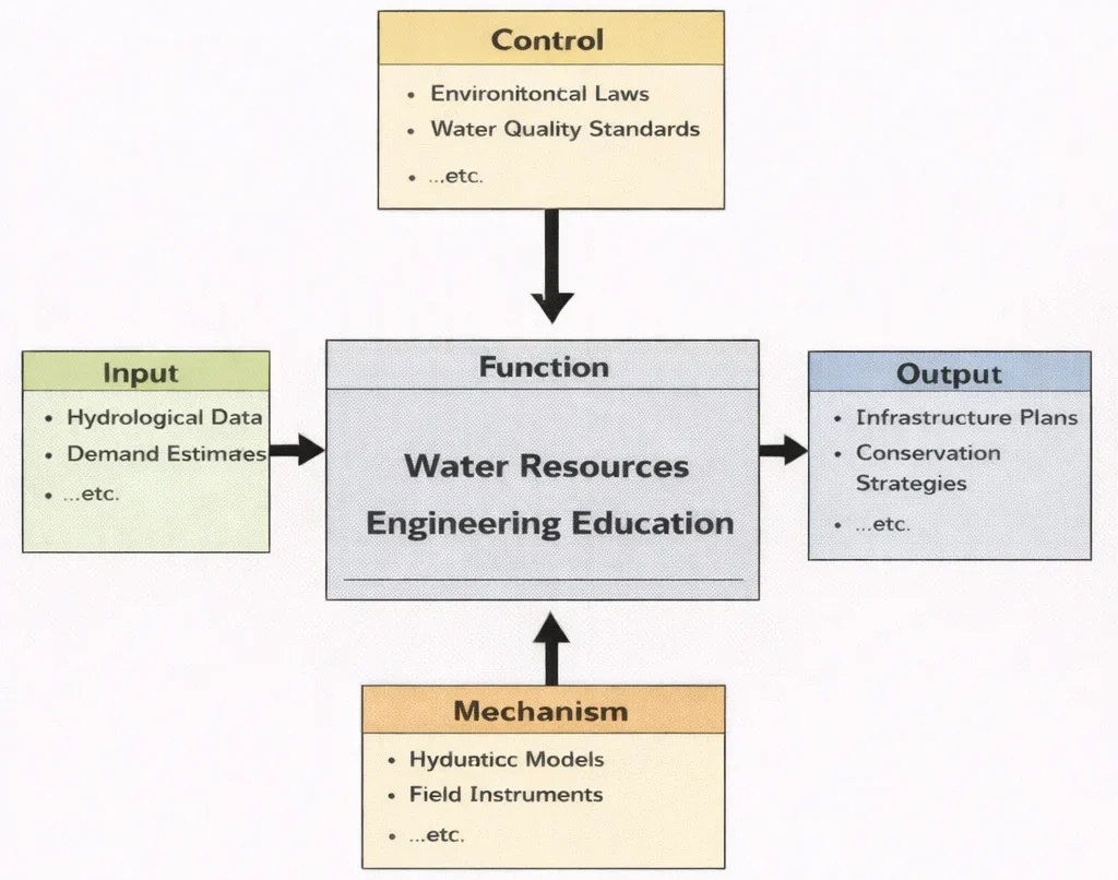
In Water Resources Engineering Education, students don’t just “wire things up”—they learn to make machines behave on purpose. The IDEF0 diagram shown below frames Water Resources Engineering Education as a discipline of translation: it takes messy, time-varying water realities—rainfall, rivers, soils, pipes, demand, and uncertainty—and turns them into decisions that can be built, operated, and trusted. The “Control” box reminds learners that water is never designed in a vacuum: standards, safety margins, legal limits, and environmental goals quietly steer every calculation and trade-off. With modelling tools, field measurements, and professional methods acting as the “Mechanism,” students learn to move from observation to prediction, and from prediction to design. What comes out is more than a set of formulas—it is the ability to shape water systems that are reliable in normal seasons and resilient when nature stops being polite.
Water Resources Engineering is a cornerstone of Environmental Engineering, focusing on the sustainable management and protection of water systems. It encompasses the design of infrastructure for water supply, flood control, drainage, irrigation, and wastewater treatment—functions that are increasingly vital as urban populations grow and climate variability intensifies. This discipline integrates both natural hydrological processes and engineered systems, demanding interdisciplinary knowledge and adaptive strategies.
- Catchment Hydrology & Runoff Mechanics: Model watershed precipitation-runoff transformations using the Rational Method, unit hydrographs, and reservoir water balance equations accounting for infiltration and evapotranspiration.
- Open-Channel & Pressurized Hydraulics: Formulate uniform flow using Manning's equation, analyze hydraulic jump dissipation and specific energy, model Darcy groundwater seepage through confined aquifers, and compute Hazen-Williams friction losses in municipal networks.
- Urban Flood Attenuation & Blue-Green Infrastructure: Evaluate detention basin level-pool routing, sponge city Low-Impact Development (LID) strategies, and membrane desalination thermodynamics (SWRO specific energy consumption).

A key concern in water management today is the impact of climate dynamics, addressed through collaborations with Climate Change Mitigation and Adaptation experts. Engineers must anticipate altered rainfall patterns, rising sea levels, and increased stormwater runoff, adjusting designs accordingly. Such foresight is also supported by insights from Environmental Monitoring and Data Analysis, which leverages sensor networks and modeling tools to track hydrologic variables in real time.
Water Resources Engineering also intersects with Air Quality Engineering and Waste Management Engineering, as contaminated runoff and landfill leachates can affect both atmospheric and aquatic environments. Coordinated systems design ensures water quality while supporting sanitation goals. In tandem, efforts in Green Building and Sustainable Design increasingly incorporate rainwater harvesting, greywater reuse, and permeable landscaping into built environments.
Natural systems play a vital role, too. Concepts from Ecological Engineering guide the development of constructed wetlands, riparian buffers, and habitat restoration projects that complement traditional infrastructure. These nature-based solutions are particularly effective in urban resilience strategies. Meanwhile, Environmental Policy and Management provides the regulatory and governance framework within which such projects must operate.
The energy-water nexus also brings this field into dialogue with Renewable Energy Systems Engineering, as hydroelectric dams, pumped storage, and desalination plants link water systems with power generation. Efficient water use in industrial contexts benefits from principles in Energy and Resource Efficiency in Manufacturing and innovations in Advanced Materials.
Digitization is transforming water infrastructure. Tools from Digital Twin Technology and Computer-Integrated Manufacturing are now being applied to real-time simulations and predictive maintenance in water distribution systems. These developments often borrow techniques from Signal Processing to analyze sensor data and optimize flow control.
Interactive System Dynamics: Storm Runoff Hydrograph & Detention Basin Attenuation
Simulate catchment storm runoff and detention basin flood routing across a 24-hour storm cycle. Adjust rainfall intensity, urban imperviousness, and detention basin capacity to observe peak discharge attenuation and flood hydrograph flattening in real time.
Hydrological Parameters
Water Resources Engineering: Curriculum Roadmap & Cluster Navigation
Explore where Water Resources Engineering fits within the broader Environmental Engineering curriculum framework. Each card outlines strategic relationships and learning objectives across related disciplines:
Environmental Engineering – Overview
Serves as the foundational hub connecting physical, biological, and chemical engineering principles across air, water, land, and urban systems.
Air Quality Engineering
Focuses on atmospheric pollutant transport, dispersion modeling, aerosol dynamics, and stack emission controls.
Water Resources Engineering (Current Page)
Integrates catchment hydrology, open-channel hydraulics, municipal water distribution, flood risk management, and groundwater flow modeling.
Waste Management Engineering
Addresses municipal solid waste handling, landfill liner engineering, toxic leachate containment, and material recycling systems.
Renewable Energy Systems Engineering
Explores the energy-water nexus, including hydroelectric dam generation, pumped-storage power, and solar-powered desalination facilities.
Industrial Ecology & Circular Economy
Promotes industrial water cascading, closed-loop wastewater recovery, and zero-liquid-discharge (ZLD) manufacturing systems.
Green Building & Sustainable Design
Incorporates urban rainwater harvesting, greywater recycling, bioswales, and permeable pavements into sustainable building design.
Environmental Policy & Management
Enforces river basin governance, water rights allocation, transboundary agreements, and regulatory quality compliance.
Environmental Monitoring & Data Analysis
Leverages real-time telemetry, river gauge sensor networks, and GIS spatial mapping for predictive hydrological forecasting.
Ecological Engineering
Utilizes constructed wetlands, re-naturalized river corridors, and living shorelines for passive water filtration and flood attenuation.
Climate Change Mitigation & Adaptation
Prepares civil infrastructure for sea-level rise, intensified extreme storm surges, and changing seasonal snowpack runoff dynamics.
Core Areas of Water Resources Engineering
Hydrology
Hydrology evaluates the global circulation, distribution, and chemical properties of terrestrial water. Civil engineers analyze the hydrologic balance equation (\(P - R - G - E - T = \Delta S\)) across catchment boundaries to predict seasonal reservoir inflows, track snowpack ablation, and determine safe groundwater pumping yields without triggering land subsidence.
Hydraulics
Hydraulics applies fluid mechanics to convey water through open channels, culverts, pressurized conduits, and hydraulic structures. Key topics include uniform flow (Manning's formula), gradually varied flow profiles (backwater curves via the direct step method), and rapidly varied flow phenomena such as hydraulic jumps at spillway aprons.
Water Supply and Distribution Systems
Municipal water delivery requires reliable conveyance from surface intakes or deep boreholes to customer taps. Engineers design transmission mains, booster pumping stations, elevated water towers for emergency fire flow, and looped pipe distributions, modeling head losses via Hazen-Williams or Darcy-Weisbach formulations.
Water Quality and Treatment Systems
Potable water facilities implement sequential multi-barrier purification: rapid coagulant flash-mixing, flocculator floc growth, sedimentation clarification, dual-media rapid sand filtration, and disinfection (chlorination, ozonation, UV irradiation) to meet statutory drinking water standards.
Flood Control and Resilient Drainage
Engineers blend structural works (levees, dikes, retention reservoirs, bypass floodways) with non-structural strategies (floodplain zoning, hydraulic early-warning telemetry, and nature-based sponge city infrastructure) to protect communities.
Problem Formulation: Rectangular Spillway Chute Critical Depth, Froude Regimes & Stilling Basin Energy Loss
A rectangular concrete floodway chute of width \(b = 6.00\text{ m}\) discharges a design flow rate \(Q = 48.00\text{ m}^3\text{/s}\). At the toe of the spillway immediately upstream of the stilling basin apron, the supercritical water depth is measured at \(y_1 = 0.80\text{ m}\). Calculate the upstream flow velocity (\(v_1\)), the upstream Froude number (\(Fr_1\)), the critical flow depth (\(y_c\)), the subcritical conjugate tailwater depth (\(y_2\)) following the hydraulic jump using the Bélanger momentum equation, and the total rate of turbulent mechanical energy dissipation (\(\Delta E\) and \(P_{\text{diss}}\)).
- Channel width: \(b = 6.00\text{ m}\); Design flow rate: \(Q = 48.00\text{ m}^3\text{/s}\)
- Unit discharge: \(q = \frac{Q}{b} = \frac{48.00}{6.00} = 8.00\text{ m}^2\text{/s}\)
- Initial supercritical depth: \(y_1 = 0.80\text{ m}\); Acceleration of gravity: \(g = 9.81\text{ m/s}^2\)
- Water density: \(\rho = 1,000.0\text{ kg/m}^3\)
Step 1: Upstream Flow Velocity (\(v_1\)) and Froude Number (\(Fr_1\))
$$v_1 = \frac{q}{y_1} = \frac{8.00\text{ m}^2\text{/s}}{0.80\text{ m}} = \mathbf{10.00\text{ m/s}}$$ $$Fr_1 = \frac{v_1}{\sqrt{g \cdot y_1}} = \frac{10.00\text{ m/s}}{\sqrt{9.81\text{ m/s}^2 \times 0.80\text{ m}}} = \frac{10.00}{\sqrt{7.848}} = \frac{10.00}{2.8014} = \mathbf{3.570}$$(Since \(Fr_1 = 3.570 \gt 1.0\), the upstream flow is confirmed to be supercritical in the stable oscillating jump regime).
Step 2: Critical Depth (\(y_c\)) and Minimum Specific Energy (\(E_{\text{min}}\))
$$y_c = \sqrt[3]{\frac{q^2}{g}} = \sqrt[3]{\frac{(8.00)^2}{9.81}} = \sqrt[3]{\frac{64.00}{9.81}} = \sqrt[3]{6.5240} = \mathbf{1.8685\text{ m}}$$ $$E_{\text{min}} = \frac{3}{2} y_c = 1.5 \times 1.8685\text{ m} = \mathbf{2.8028\text{ m}}$$Step 3: Subcritical Conjugate Depth (\(y_2\)) via the Bélanger Equation
$$y_2 = \frac{y_1}{2} \left( \sqrt{1 + 8 \cdot Fr_1^2} - 1 \right)$$ $$y_2 = \frac{0.80}{2} \left( \sqrt{1 + 8 \times (3.570)^2} - 1 \right) = 0.40 \left( \sqrt{1 + 8 \times 12.7449} - 1 \right)$$ $$y_2 = 0.40 \left( \sqrt{1 + 101.959} - 1 \right) = 0.40 \left( \sqrt{102.959} - 1 \right) = 0.40 (10.1469 - 1) = 0.40 \times 9.1469 = \mathbf{3.6588\text{ m}}$$Step 4: Specific Energy Loss (\(\Delta E\)) & Total Power Dissipated (\(P_{\text{diss}}\))
Calculate the head loss across the jump using the rectangular channel formula:
$$\Delta E = \frac{(y_2 - y_1)^3}{4 \cdot y_1 \cdot y_2} = \frac{(3.6588 - 0.80)^3}{4 \times 0.80 \times 3.6588} = \frac{(2.8588)^3}{11.7082} = \frac{23.3642}{11.7082} = \mathbf{1.9955\text{ meters of head}}$$Compute continuous hydrodynamic power converted to turbulence and heat:
$$P_{\text{diss}} = \rho \cdot g \cdot Q \cdot \Delta E = 1,000\text{ kg/m}^3 \times 9.81\text{ m/s}^2 \times 48.00\text{ m}^3\text{/s} \times 1.9955\text{ m}$$ $$P_{\text{diss}} = 470,880.0 \times 1.9955 = \mathbf{939,641\text{ Watts}}\quad (\mathbf{939.64\text{ kW}}\text{ or }\mathbf{0.940\text{ MW}})$$Systems Engineering Trade-Off Matrix: Water Infrastructure & Supply Technologies
Selecting municipal water supply and flood mitigation strategies requires balancing volumetric yield reliability, capital expenditures, operational energy draw, land footprints, and climate resilience.
| Infrastructure Modality | Primary Mechanism | Volumetric Supply Reliability | CAPEX vs. OPEX Energy Draw | Environmental & Ecological Risks | Climate Resilience Factor |
|---|---|---|---|---|---|
| Surface Water Reservoirs | Gravity dam impoundment of river catchment runoff | High seasonal capacity; vulnerable to multi-year droughts | High upfront CAPEX; very low operational pumping cost | Riparian habitat flooding; sediment trapping and river fragmentation | Moderate; susceptible to evaporation and changing snowpack |
| Seawater Reverse Osmosis (SWRO) | High-pressure membrane separation across semipermeable barriers | Infinite ocean supply; 100% weather independent | High CAPEX; energy intensive (\(2.5 - 3.8\text{ kWh/m}^3\)) | Hypersaline brine discharge; marine larval entrainment at intake | Exceptional; complete immunity to meteorological droughts |
| Managed Aquifer Recharge (MAR) | Infiltration basins & deep borehole water injection | Sub-surface seasonal bank storage; zero evaporative loss | Low CAPEX; modest pumping and pre-treatment OPEX | Clogging of well screens; potential aquifer contamination | High; underground storage buffers against extreme heat waves |
| Sponge City Blue-Green SUDS | Permeable paving, bioswales, retention wetlands | Decentralized stormwater capture; urban flood mitigation | Distributed civil cost; replaces expensive storm pipe upgrades | Net ecological gain; urban biodiversity and microclimate cooling | High; absorbs flash rainfall and reduces urban heat island spikes |
| Indirect Potable Reuse (IPR) | Microfiltration, reverse osmosis, UV advanced oxidation | Continuous municipal baseline; matches urban wastewater flows | Moderate-to-high CAPEX; lower energy than SWRO (\(1.2 - 2.0\text{ kWh/m}^3\)) | Public perception barriers; trace micropollutant monitoring required | Very high; establishes closed circular water loops for cities |
Applications of Water Resources Engineering
- Municipal Water Distribution Networks: Hydraulic transient modeling manages water hammer pressure surges, while automated district metered areas (DMAs) cut non-revenue water (NRW) pipe leaks by 25%.
- Agricultural Irrigation Efficiency: Precision drip networks and evapotranspiration-based irrigation scheduling conserve freshwater while preventing soil salinization.
- Industrial Zero-Liquid-Discharge (ZLD): Membrane filtration combined with brine crystallizers recovers over 95% of industrial process water, protecting municipal sewer systems.
- Regional Flood Routing & Early Warning: Coupled 1D/2D hydrodynamic models (e.g., HEC-RAS, MIKE FLOOD) translate Doppler radar rainfall into real-time inundation maps to direct emergency civil defenses.
- Coastal Storm Surge Barriers: Automated tidal gates, sea dikes, and living mangrove revetments protect low-lying coastal deltas from storm tides and rising sea levels.
Why Study Water Resources Engineering
Securing Global Freshwater Supplies
Students design systems that deliver potable water to expanding cities, balance competing agricultural and industrial claims, and protect aquatic baseflows.
Hydraulic and Hydrologic Computational Mastery
Engineers gain hands-on proficiency with industry tools (HEC-HMS, HEC-RAS, EPA-SWMM, EPANET) to simulate extreme storm runoff, river hydraulics, and pressurized networks.
Civil Infrastructure Flood Resilience
Coursework covers the design of dams, spillways, detention ponds, stilling basins, and nature-based sponge city infrastructure capable of withstanding extreme storms.
Integrated Basin Governance (IWRM)
Students examine water rights allocation, transboundary river treaties, and regulatory quality frameworks to resolve inter-sectoral resource competition.
Water Resources Engineering: Conclusion
Water Resources Engineering provides the technical foundation for safeguarding human civilization and natural aquatic ecosystems against hydrological volatility. By linking catchment hydrology and fluid mechanics with digital twin telemetry and nature-based infrastructure, engineers turn chaotic weather extremes into predictable, managed systems. As climate change, population growth, and aquifer depletion challenge traditional water resources, the discipline offers the predictive modeling tools, infrastructure designs, and governance strategies needed to secure a sustainable water future.
Frequently Asked Questions
How do the main processes of the hydrological cycle guide water engineering design?
Precipitation depth and frequency establish design storm volumes; infiltration rates determine runoff hydrographs; evapotranspiration governs reservoir losses and irrigation demands; and groundwater baseflow sustains river ecosystems during dry periods.
What is the difference between detention and retention basins in stormwater management?
Detention basins ("dry ponds") temporarily store peak runoff and release it through a controlled orifice to reduce downstream flooding. Retention basins ("wet ponds") maintain a permanent pool that provides long-term biological settling and water quality treatment.
How does Managed Aquifer Recharge (MAR) prevent land subsidence and coastal saltwater intrusion?
MAR injects surface water or treated reclaimed water into depleted aquifers via infiltration basins or injection wells. Restoring pore water pressure prevents aquifer compaction, halts land subsidence, and maintains a hydraulic barrier against inland saltwater intrusion.
End-of-Page Practice & Assessment Modules
Section 1: Interactive Foundational Concepts Review
Question 1: Hydrologic Stationarity Invalidation under Climate Shifts
Question 2: Open-Channel vs. Pressurized Conduit Fluid Mechanics
Question 3: Integrated Water Resources Management (IWRM) Core Principles
Question 4: Water Quality Multi-Barrier Treatment Approach
Section 2: Analytical & Scenario-Based Inquiry
Question 1: Mitigating Urban Runoff Peak Amplification via SUDS
Question 2: Transboundary River Basin Negotiation & Joint Modeling
Question 3: Digital Twin Implementation in Municipal Water Distribution
Section 3: Applied Engineering Quantitative Calculations
Problem 1: Rational Method Peak Storm Runoff Discharge
Question: An urban catchment has an area \(A = 25.0\text{ hectares}\) (\(250,000.0\text{ m}^2\)). The catchment consists of \(60.0\%\) impervious surfaces (\(C_1 = 0.90\)) and \(40.0\%\) permeable parkland (\(C_2 = 0.25\)). For a 10-year storm, rainfall intensity is \(I = 72.0\text{ mm/hr}\). Calculate the composite runoff coefficient \(C_{\text{comp}}\) and the peak storm discharge \(Q_{\text{peak}}\) in \(\text{m}^3\text{/s}\).
Solution:
1. Composite runoff coefficient:
$$C_{\text{comp}} = (0.60 \times 0.90) + (0.40 \times 0.25) = 0.54 + 0.10 = \mathbf{0.640}$$2. Convert rainfall intensity to meters per second:
$$I = \frac{72.0\text{ mm/hr}}{1,000.0 \times 3,600.0} = 2.00 \times 10^{-5}\text{ m/s}$$3. Peak discharge via the Rational Method:
$$Q_{\text{peak}} = C_{\text{comp}} \cdot I \cdot A = 0.640 \times (2.00 \times 10^{-5}\text{ m/s}) \times 250,000.0\text{ m}^2 = \mathbf{3.20\text{ m}^3\text{/s}}$$Problem 2: Manning's Equation Open Channel Hydraulic Capacity
Question: A rectangular concrete stormwater channel has a bed width \(b = 3.00\text{ m}\), flow depth \(y = 1.20\text{ m}\), and longitudinal slope \(S_0 = 0.0015\). Using Manning’s roughness coefficient \(n = 0.013\), calculate the flow area \(A\), wetted perimeter \(P\), hydraulic radius \(R_h\), and uniform discharge capacity \(Q\) in \(\text{m}^3\text{/s}\).
Solution:
1. Geometric properties:
$$A = b \cdot y = 3.00\text{ m} \times 1.20\text{ m} = 3.60\text{ m}^2$$ $$P = b + 2y = 3.00\text{ m} + 2(1.20\text{ m}) = 5.40\text{ m}$$ $$R_h = \frac{A}{P} = \frac{3.60\text{ m}^2}{5.40\text{ m}} = 0.6667\text{ m}$$2. Flow discharge capacity via Manning's formula:
$$Q = \frac{1}{n} \cdot A \cdot R_h^{2/3} \cdot S_0^{1/2} = \frac{1}{0.013} \times 3.60 \times (0.6667)^{2/3} \times (0.0015)^{1/2}$$ $$Q = 76.923 \times 3.60 \times 0.7631 \times 0.03873 = \mathbf{8.18\text{ m}^3\text{/s}}$$Problem 3: Darcy's Law Confined Aquifer Groundwater Seepage
Question: A confined sand aquifer has a hydraulic conductivity \(K = 25.0\text{ m/day}\) and thickness \(b = 12.0\text{ m}\). Two piezometers spaced \(L = 500.0\text{ m}\) apart along the flow path measure heads \(h_1 = 45.0\text{ m}\) and \(h_2 = 41.0\text{ m}\). Across an aquifer width \(W = 1,000.0\text{ m}\), calculate the hydraulic gradient \(i\) and daily groundwater discharge \(Q\) in \(\text{m}^3\text{/day}\).
Solution:
1. Hydraulic gradient:
$$i = \frac{h_1 - h_2}{L} = \frac{45.0\text{ m} - 41.0\text{ m}}{500.0\text{ m}} = \frac{4.0}{500.0} = \mathbf{0.0080}$$2. Cross-sectional flow area: \(A = W \cdot b = 1,000.0\text{ m} \times 12.0\text{ m} = 12,000.0\text{ m}^2\)
3. Total daily groundwater discharge:
$$Q = K \cdot i \cdot A = 25.0\text{ m/day} \times 0.0080 \times 12,000.0\text{ m}^2 = \mathbf{2,400.0\text{ m}^3\text{/day}}$$Problem 4: Hazen-Williams Water Main Friction Head Loss
Question: A ductile iron municipal water main (\(D = 0.30\text{ m}\), roughness coefficient \(C = 120\)) conveys a drinking water flow rate \(Q = 0.080\text{ m}^3\text{/s}\) over length \(L = 1,500.0\text{ m}\). Calculate friction head loss \(h_f\) in meters using the empirical formulation: \(h_f = \frac{10.67 \cdot L \cdot Q^{1.852}}{C^{1.852} \cdot D^{4.87}}\).
Solution:
1. Calculate numerator:
$$\text{Num} = 10.67 \times 1,500.0 \times (0.080)^{1.852} = 16,005.0 \times 0.0091873 = 147.043$$2. Calculate denominator:
$$\text{Den} = (120)^{1.852} \times (0.30)^{4.87} = 7,020.24 \times 0.0028213 = 19.806$$3. Total frictional head loss:
$$h_f = \frac{147.043}{19.806} = \mathbf{7.42\text{ meters of head}}$$Problem 5: Reservoir Water Balance Storage Mass Balance
Question: A reservoir begins a monthly billing period with initial storage \(S_0 = 5,000,000.0\text{ m}^3\). Over the month, stream inflow is \(I = 1,200,000.0\text{ m}^3\), rainfall onto the surface is \(P = 80,000.0\text{ m}^3\), surface evaporation is \(E = 150,000.0\text{ m}^3\), municipal withdrawal is \(W = 900,000.0\text{ m}^3\), and mandatory environmental flow release is \(R = 100,000.0\text{ m}^3\). Calculate end-of-month storage \(S_1\) in \(\text{m}^3\).
Solution:
1. Apply the conservation of mass water balance:
$$S_1 = S_0 + I + P - E - W - R$$ $$S_1 = 5,000,000.0 + 1,200,000.0 + 80,000.0 - 150,000.0 - 900,000.0 - 100,000.0$$ $$S_1 = 6,280,000.0 - 1,150,000.0 = \mathbf{5,130,000.0\text{ m}^3}$$Problem 6: Rapid Sand Filter Hydraulic Loading Area Sizing
Question: A drinking water treatment plant treats a flow \(Q = 28,800.0\text{ m}^3\text{/day}\) distributed across four identical parallel rapid sand filter beds. The maximum allowable filtration velocity is \(v = 5.0\text{ m/hr}\) (\(120.0\text{ m/day}\)). Calculate the total required filter surface area \(A_{\text{total}}\) and the area required per bed \(A_{\text{bed}}\) in \(\text{m}^2\).
Solution:
1. Total filter area:
$$A_{\text{total}} = \frac{Q}{v} = \frac{28,800.0\text{ m}^3\text{/day}}{120.0\text{ m/day}} = \mathbf{240.0\text{ m}^2}$$2. Area per individual filter bed (\(N = 4\)):
$$A_{\text{bed}} = \frac{240.0\text{ m}^2}{4} = \mathbf{60.0\text{ m}^2\text{ per bed}}$$Problem 7: Seawater Reverse Osmosis (SWRO) Desalination Power Draw
Question: A municipal SWRO plant produces \(10,000.0\text{ m}^3\text{/day}\) of potable water from seawater at recovery ratio \(Y = 45.0\%\). The high-pressure pump operates at net feed pressure \(P = 60.0\text{ bar}\) (\(6,000,000.0\text{ Pa}\)) with pump efficiency \(\eta = 0.85\). An energy recovery device (ERD) reduces specific pumping energy by \(40.0\%\). Determine the required intake flow rate \(Q_{\text{feed}}\) and total daily electrical energy consumed in \(\text{kWh/day}\).
Solution:
1. Required intake seawater feed flow rate:
$$Q_{\text{feed}} = \frac{Q_{\text{product}}}{Y} = \frac{10,000.0\text{ m}^3\text{/day}}{0.45} = 22,222.22\text{ m}^3\text{/day} = 0.2572\text{ m}^3\text{/s}$$2. Baseline pump hydraulic power:
$$P_{\text{base}} = \frac{Q_{\text{feed}} \cdot P}{\eta} = \frac{0.2572\text{ m}^3\text{/s} \times 6,000,000.0\text{ Pa}}{0.85} = \frac{1,543,200.0\text{ W}}{0.85} = 1,815.53\text{ kW}$$3. Net power accounting for 40% ERD energy recovery:
$$P_{\text{net}} = 1,815.53\text{ kW} \times (1.0 - 0.40) = 1,089.32\text{ kW}$$4. Total daily electricity consumption:
$$E_{\text{daily}} = 1,089.32\text{ kW} \times 24.0\text{ hr} = \mathbf{26,143.68\text{ kWh/day}}\quad (\text{Specific Energy} \approx 2.61\text{ kWh/m}^3)$$