
Emerging technologies education is not only about tracking what is newly invented, but about learning how to evaluate technological change systematically. Technological breakthroughs, market pressures, and scientific inquiries serve as inputs, while empirical evidence and physical first principles act as the governing controls that prevent hype from replacing rigorous validation. Supported by quantitative data, open benchmarks, and grounded case studies, learners develop the capacity to analyze emerging systems, assess realistic operational capabilities, anticipate socio-technical trade-offs, and compare competing solutions through structured reasoning.
Emerging technologies represent the critical transition zone between foundational scientific discovery and mature, large-scale engineering deployment. Unlike standardized commercial infrastructure, emerging systems are actively evolving in form, interfacial protocols, material constraints, and regulatory policies. This page serves as a master conceptual hub within the STEM curriculum, guiding students through how frontier technologies originate, cross disciplinary boundaries, and gradually transform industry and global infrastructure.
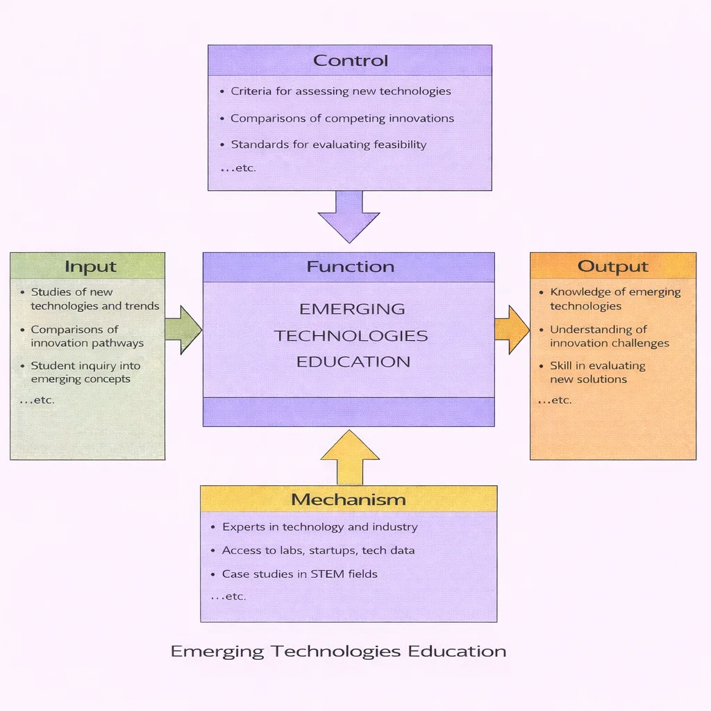
At their foundation, emerging technologies operate as cross-disciplinary cyber-physical systems rather than isolated laboratory artifacts. They rely on algebraic formalisms from pure and applied mathematics, stochastic probability from statistics, distributed architectures from information technology, and high-dimensional optimization from data science and analytics. These quantitative foundations directly support frontiers such as biotechnology, intelligent autonomous robotics, and solid-state quantum devices.
A defining characteristic of an emerging technology is its capacity to reframe problem-solving paradigms rather than merely offering incremental performance improvements. Quantum computing exemplifies this paradigm shift: by exploiting linear combinations in quantum superposition and non-local correlations in quantum entanglement via physical qubits and unitary quantum circuits, it bypasses classical Turing complexity constraints for specific mathematical problem classes.
Concurrently, physical embodiment and autonomy represent a major axis of innovation. Modern autonomous robotics and swarm systems unite onboard computer vision, state estimation, and dynamic feedback control over distributed telemetry networks. Connectivity scales these systems from benchtop prototypes to physical ecosystems via the Internet of Things (IoT) and Industry 4.0 smart manufacturing platforms.
Simultaneously, innovation centers on planetary resilience and off-world expansion. Developments in renewable energy and grid-scale battery storage, sustainable materials design, and environmental remediation address terrestrial resource limits, while space exploration technologies and reusable launch vehicles transition orbital mechanics into permanent commercial infrastructure.

Core Disciplinary Domains in Frontier Technologies
Emerging technologies can be systematically categorized into four core domains, each reflecting a foundational methodology for addressing complex physical and computational challenges:
Autonomous Systems & Robotics →
Systems engineered to perceive dynamic unstructured environments, execute real-time state estimation, and close actuation feedback loops with minimal human oversight. Forms the foundation of mobile robotics, autonomous vehicles, and distributed swarm architectures.
Destination URL: https://prep4uni.online/stem/emerging-technologies/autonomous-systems/Synthetic Biology & Biotechnology →
Engineering living systems and biochemical pathways through targeted genetic editing, automated cellular assays, and metabolic engineering. Applications span molecular therapeutics, targeted agricultural resilience, and synthetic biomaterials.
Destination URL: https://prep4uni.online/stem/emerging-technologies/biotechnology/Quantum Information Science →
Computational mechanics operating on quantum phenomena—specifically state superposition, phase interference, and quantum entanglement. Unlocks exponential speedups for integer factorization, discrete optimization, and molecular simulation.
Destination URL: https://prep4uni.online/stem/emerging-technologies/quantum-computing/Space Exploration & Orbital Systems →
Engineering frameworks supporting extended space operations, including high-thrust staged-combustion rocket engines, autonomous satellite constellation networking, closed-loop environmental control, and in-situ planetary resource utilization.
Destination URL: https://prep4uni.online/stem/emerging-technologies/space-exploration-technologies/How Frontier Innovations Cross Disciplinary Boundaries
Emerging technologies rarely stay confined to their originating discipline. Instead, methodologies migrate across domains through three primary systemic pathways:
Methodological Evaluation: Distinguishing Hype from Operational Reality
Emerging technologies often attract exaggerated performance claims and premature commercialization timelines. Developing technical maturity requires applying a systematic evaluation rubric based on four foundational diagnostic tests:
- The Demonstration Gap: Evaluate whether a system operates reliably only under pristine, highly controlled laboratory parameters, or whether it demonstrates robustness against stochastic sensor noise, non-deterministic environmental factors, and degraded communication links.
- The Cost of Operating Conditions: Examine whether technical viability depends on fragile, economically unsustainable environmental controls—such as dilution refrigeration at \(15 \text{ mK}\), ultra-high vacuum chambers, or pure chemical feedstocks—that limit field scalability.
- Comparative Baseline Validity: Verify claims against state-of-the-art classical baselines tested under equivalent operational, thermal, and computational constraints, rather than comparing against obsolete or unoptimized legacy algorithms.
- Ecosystem and Infrastructure Signals: Monitor the emergence of formal international standards (IEEE, ISO), interoperable open-source software libraries, reproducible test benchmarks, and institutional safety regulations.
Interactive Technology Readiness Level (TRL) & Maturity Dynamics
The NASA/ISO Technology Readiness Level (TRL) scale benchmarks innovation maturity from basic physical principles (TRL 1) to flight-proven, commercial operation (TRL 9). Use this dynamic simulator to examine how investment velocity and research constraints alter development timelines:
Professional Roles & Engineering Trajectories in Frontier Sectors
Frontier engineering domains demand specialized mathematical proficiency, software competence, and empirical rigor:
| Specialized Track | Core Technical Competency | Primary Tools & Methodologies | Typical Industrial Destination |
|---|---|---|---|
| Autonomous Systems Specialist | State estimation, dynamic obstacle avoidance, non-holonomic kinematics, multi-agent consensus | ROS 2, C++, Extended Kalman Filtering (EKF), Point Cloud Library (PCL), Control Barrier Functions | Warehouse AMR fleets, autonomous commercial aviation, mining robotics |
| Biotechnology Innovator | CRISPR-Cas9 design, automated bioreactor optimization, molecular cloning, metabolomics | Next-Generation Sequencing (NGS), BioPython, microfluidic chips, mass spectrometry | Therapeutic biomanufacturing, agricultural gene editing, synthetic biomaterials |
| Quantum Information Scientist | Quantum circuit compilation, error-correcting surface codes, Hamiltonian simulation | Qiskit, Cirq, dilutive cryogenics, microwave pulse engineering, Lie groups | Quantum computing hardware labs, post-quantum cryptography, financial quant research |
| Space Systems Engineer | Orbital mechanics, structural aerothermal analysis, regenerative cooling, space avionics | GMAT, STK, finite element thermal modeling, radiation-hardened RTOS, optical communications | Commercial launch providers, orbital payload servicing, deep-space exploration agencies |
Frequently Asked Questions on Emerging Technologies in STEM
1. What criteria distinguish an emerging technology from a mature engineering system?
Emerging technologies are characterized by active paradigm evolution, non-standardized architectures, uncertain regulatory and safety frameworks, and a performance profile transitioning between proof-of-concept and commercial viability. Mature systems operate with established international codes, predictable supply chains, and standardized manufacturing tolerances.
2. Why is cross-disciplinary literacy vital for studying emerging fields?
Frontier systems rarely inhabit single disciplines. For example, quantum computing requires solid-state physics for physical qubit stability, microwave engineering for gate pulses, and pure mathematics for quantum algorithms. Without cross-disciplinary literacy, engineers struggle to address bottlenecks outside their narrow specialization.
3. How does quantum computing surpass classical Von Neumann computer architecture?
Classical computers represent states as deterministic binary bits (\(0\) or \(1\)). Quantum computers utilize quantum two-level systems (qubits) capable of continuous complex linear superpositions. An \(n\)-qubit quantum register can represent \(2^n\) complex probability amplitudes concurrently, enabling quantum algorithms to solve specific combinatorial and quantum chemistry problems exponentially faster than classical supercomputers.
4. What engineering hurdles limit the deployment of magnetic confinement nuclear fusion?
Tokamak and stellarator fusion reactors require sustaining hydrogen plasmas at temperatures exceeding \(100 \times 10^6 \text{ K}\) using strong magnetic confinement fields while preventing plasma turbulence and instabilities. Key challenges include developing neutron-resistant divertor wall materials and breeding tritium fuel within lithium blankets to achieve sustained net electrical energy gain (\(Q_{\text{electric}} \gt 1\)).
Interactive Self-Assessment: Conceptual Verification
Select any question below to expand the detailed technical explanation:
1. How do emerging technologies differ from mature established systems?
2. Why is CRISPR-Cas9 categorized as an emerging biotechnology?
3. What distinguishes an autonomous system from a traditional automated industrial system?
4. How does a cyber-physical smart grid optimize renewable energy integration?
5. Why is nanoelectronics essential for extending computing performance beyond classical silicon limits?
End-of-Page Comprehensive Practice Module
Part I: Foundational Concepts & Direct Review
1. Define the role of an IDEF0 functional diagram in systems engineering education.
2. What is tool migration in the context of interdisciplinary STEM evolution?
3. Contrast quantum state superposition with quantum entanglement.
4. What does the demonstration gap measure during technology evaluation?
5. How do closed-loop life-support systems (ECLSS) enable long-duration space travel?
Part II: Analytical & Scenario-Based Inquiry
1. How does nuclear fusion fundamentally differ from nuclear fission in waste and fuel safety?
2. What failure modes threaten safety-critical autonomous systems in unmodeled edge environments?
3. How does problem migration accelerate innovation between biotechnology and semiconductor lithography?
4. Why do open-source software libraries serve as early indicators of technological maturity?
Part III: Step-by-Step Quantitative Computations
Problem 1: Quantum Hilbert Space Dimensionality Sizing
Scenario: A quantum computational register contains \(n = 10\) entangled physical qubits. Calculate the dimension of the complex state vector space that this register represents simultaneously in superposition.
Step-by-Step Derivation:
$$ \begin{aligned} \text{State Space Dimension } D &= 2^n \\ D &= 2^{10} = 1{,}024 \text{ simultaneous complex amplitudes} \end{aligned} $$Answer & Conclusion: A 10-qubit quantum register spans a state Hilbert space of exactly 1,024 simultaneous orthogonal states.
Problem 2: Exponential Register Expansion Scaling
Scenario: An experimental quantum processor is upgraded by adding 4 additional qubits, increasing its register from \(n_1 = 10\) to \(n_2 = 14\) qubits. Compute the exact multiplicative increase in the register's simultaneous computational capacity.
Step-by-Step Derivation:
$$ \begin{aligned} D_1 &= 2^{10} = 1{,}024 \\ D_2 &= 2^{14} = 16{,}384 \\ \text{Capacity Expansion Ratio } R &= \frac{D_2}{D_1} = \frac{2^{14}}{2^{10}} = 2^{14 - 10} = 2^4 = 16 \end{aligned} $$Answer & Conclusion: Adding 4 qubits increases state capacity by a factor of \(16\times\).
Problem 3: Dead-Reckoning Odometry Drift Uncertainty
Scenario: An autonomous planetary rover traverses a straight trajectory of \(d = 120.0 \text{ m}\) without external visual or satellite fixes. Wheel slippage causes position error to accumulate at an empirical rate of \(\epsilon = 0.05 \text{ m}\) per meter traveled. Calculate the final position uncertainty \(\Delta x\).
Step-by-Step Derivation:
$$ \begin{aligned} \Delta x &= d \times \epsilon \\ \Delta x &= 120.0 \text{ m} \times 0.05 \text{ m}\cdot\text{m}^{-1} = 6.0 \text{ m} \end{aligned} $$Answer & Conclusion: The rover accumulates an operational position uncertainty of \(6.0 \text{ m}\), demonstrating why periodic sensor fusion resets are necessary.
Problem 4: Smart Grid Energy Transmission Efficiency
Scenario: A commercial photovoltaic installation generates \(E_{\text{gen}} = 450.0 \text{ kWh}\) daily. Energy is routed through a battery storage system with round-trip efficiency \(\eta_{\text{storage}} = 90.0\%\), followed by distribution over a microgrid with transmission losses of \(L = 5.0\%\) (\(\eta_{\text{trans}} = 95.0\%\)). Determine the net energy delivered to the consumer.
Step-by-Step Derivation:
$$ \begin{aligned} E_{\text{stored}} &= E_{\text{gen}} \times \eta_{\text{storage}} = 450.0 \text{ kWh} \times 0.90 = 405.0 \text{ kWh} \\ E_{\text{net}} &= E_{\text{stored}} \times \eta_{\text{trans}} = 405.0 \text{ kWh} \times 0.95 = 384.75 \text{ kWh} \end{aligned} $$Answer & Conclusion: Net delivered energy equals \(384.75 \text{ kWh}\), reflecting an overall system efficiency of \(85.5\%\).
Problem 5: Orbital Period Reduction & Daily Pass Sizing
Scenario: A remote-sensing satellite in Low Earth Orbit (LEO) completes \(N_0 = 16\) revolutions per \(24.0\text{-hour}\) day (\(1{,}440.0 \text{ min}\)). An electric propulsion burn shifts its altitude, reducing its orbital period by \(\Delta T = 6.0 \text{ minutes}\). Calculate the new orbital period and the number of complete revolutions completed every \(24.0 \text{ hours}\).
Step-by-Step Derivation:
$$ \begin{aligned} T_0 &= \frac{1{,}440.0 \text{ min}}{16} = 90.0 \text{ min/orbit} \\ T_{\text{new}} &= T_0 - \Delta T = 90.0 \text{ min} - 6.0 \text{ min} = 84.0 \text{ min/orbit} \\ N_{\text{new}} &= \frac{1{,}440.0 \text{ min}}{84.0 \text{ min/orbit}} \approx 17.14 \text{ orbits} \end{aligned} $$Answer & Conclusion: The new orbital period is \(84.0 \text{ min}\), allowing the satellite to complete 17 full orbits per day.
Problem 6: Semiconductor Gate Length Scaling Percentage
Scenario: An advanced nanoelectronic fabrication process scales a transistor physical gate length down from \(L_1 = 14.0 \text{ nm}\) to \(L_2 = 2.0 \text{ nm}\). Calculate the absolute reduction and the percentage reduction in gate length.
Step-by-Step Derivation:
$$ \begin{aligned} \Delta L &= L_1 - L_2 = 14.0 \text{ nm} - 2.0 \text{ nm} = 12.0 \text{ nm} \\ \text{Percentage Reduction} &= \left( \frac{\Delta L}{L_1} \right) \times 100\% = \left( \frac{12.0}{14.0} \right) \times 100\% \approx 85.71\% \end{aligned} $$Answer & Conclusion: The process achieves an \(85.71\%\) dimensional reduction in transistor gate length.
Problem 7: Exponential Bioreactor Cellular Growth Sizing
Scenario: An automated bioprocess bioreactor cultures engineered bacterial cells with a population doubling time of \(\tau = 4.0 \text{ h}\). Starting from an initial biomass density of \(X_0 = 0.50 \text{ g}\cdot\text{L}^{-1}\), calculate the final density \(X(t)\) after \(t = 16.0 \text{ hours}\) of unconstrained exponential growth.
Step-by-Step Derivation:
$$ \begin{aligned} n_{\text{doublings}} &= \frac{t}{\tau} = \frac{16.0 \text{ h}}{4.0 \text{ h}} = 4.0 \\ X(t) &= X_0 \times 2^{n_{\text{doublings}}} = 0.50 \text{ g}\cdot\text{L}^{-1} \times 2^4 = 0.50 \times 16 = 8.0 \text{ g}\cdot\text{L}^{-1} \end{aligned} $$Answer & Conclusion: The biomass density reaches \(8.0 \text{ g}\cdot\text{L}^{-1}\) after 16 hours.
Problem 8: Grover Quantum Search Algorithmic Speedup
Scenario: A database contains \(N = 1{,}000{,}000\) unsorted entries. Classical linear search requires an average of \(N/2 = 500{,}000\) operations. Grover's quantum search algorithm finds the target entry in \(\mathcal{O}(\sqrt{N})\) oracle evaluations. Compute the quantum query count and the resulting speedup factor.
Step-by-Step Derivation:
$$ \begin{aligned} \text{Classical Average Operations } C_{\text{class}} &= \frac{1{,}000{,}000}{2} = 500{,}000 \text{ queries} \\ \text{Quantum Operations } C_{\text{quantum}} &= \sqrt{N} = \sqrt{1{,}000{,}000} = 1{,}000 \text{ queries} \\ \text{Algorithmic Speedup Factor } S &= \frac{C_{\text{class}}}{C_{\text{quantum}}} = \frac{500{,}000}{1{,}000} = 500\times \end{aligned} $$Answer & Conclusion: The quantum search algorithm requires 1,000 queries, delivering a \(500\times\) reduction in search operations.
Problem 9: Aerospace Composite Structural Mass Sizing
Scenario: A space launch vehicle stage has a baseline metallic dry mass of \(M_0 = 40{,}000.0 \text{ kg}\). Transitioning the fuselage and interstage to carbon-composite materials reduces structural mass by \(15.0\%\). Determine the mass saved and the new structural dry mass.
Step-by-Step Derivation:
$$ \begin{aligned} M_{\text{saved}} &= M_0 \times 0.15 = 40{,}000.0 \text{ kg} \times 0.15 = 6{,}000.0 \text{ kg} \\ M_{\text{final}} &= M_0 - M_{\text{saved}} = 40{,}000.0 \text{ kg} - 6{,}000.0 \text{ kg} = 34{,}000.0 \text{ kg} \end{aligned} $$Answer & Conclusion: Structural dry mass decreases to \(34{,}000.0 \text{ kg}\), saving \(6{,}000.0 \text{ kg}\) of structural mass for additional payload capacity.
Problem 10: Tokamak Plasma Confinement Duration Improvement
Scenario: An experimental magnetic confinement fusion reactor holds stable plasma for \(\tau_0 = 20.0 \text{ s}\). Upgraded high-temperature superconducting (HTS) magnets increase the confinement duration by \(250.0\%\). Calculate the new stable plasma duration.
Step-by-Step Derivation:
$$ \begin{aligned} \Delta \tau &= \tau_0 \times 2.50 = 20.0 \text{ s} \times 2.50 = 50.0 \text{ s} \\ \tau_{\text{final}} &= \tau_0 + \Delta \tau = 20.0 \text{ s} + 50.0 \text{ s} = 70.0 \text{ s} \end{aligned} $$Answer & Conclusion: The improved magnetic confinement extends stable plasma duration to \(70.0 \text{ seconds}\).
Problem 11: Edge Computer Vision Frame Rate Acceleration
Scenario: An autonomous navigation camera processes images at \(FPS_0 = 120.0 \text{ frames/s}\). TensorRT quantization reduces the per-frame inference latency by \(25.0\%\). Determine the new per-frame latency and the resulting frame processing rate.
Step-by-Step Derivation:
$$ \begin{aligned} t_{\text{frame}, 0} &= \frac{1}{120.0 \text{ s}^{-1}} \approx 0.008333 \text{ s} \quad (8.333 \text{ ms}) \\ t_{\text{frame}, \text{opt}} &= t_{\text{frame}, 0} \times (1 - 0.25) = 0.008333 \text{ s} \times 0.75 = 0.00625 \text{ s} \quad (6.25 \text{ ms}) \\ FPS_{\text{opt}} &= \frac{1}{t_{\text{frame}, \text{opt}}} = \frac{1}{0.00625 \text{ s}} = 160.0 \text{ frames/s} \end{aligned} $$Answer & Conclusion: Reducing frame latency to \(6.25 \text{ ms}\) increases throughput to 160 frames per second.
Problem 12: Optical Deep-Space Telemetry Volume Calculation
Scenario: A deep-space laser communications terminal transmits science telemetry at a continuous data rate of \(R = 250.0 \text{ Mbps}\). During an active communication window of \(t = 10.0 \text{ minutes}\), compute the total volume of data delivered in Gigabytes (GB), assuming \(1 \text{ byte} = 8 \text{ bits}\) and decimal metric units (\(1 \text{ GB} = 10^9 \text{ bytes}\)).
Step-by-Step Derivation:
$$ \begin{aligned} t_{\text{sec}} &= 10.0 \text{ min} \times 60 \text{ s}\cdot\text{min}^{-1} = 600.0 \text{ s} \\ \text{Total Megabits} &= 250.0 \text{ Mbits}\cdot\text{s}^{-1} \times 600.0 \text{ s} = 150{,}000.0 \text{ Mbits} \\ \text{Total Megabytes} &= \frac{150{,}000.0 \text{ Mbits}}{8 \text{ bits/byte}} = 18{,}750.0 \text{ MB} \\ \text{Total Gigabytes} &= \frac{18{,}750.0 \text{ MB}}{1{,}000} = 18.75 \text{ GB} \end{aligned} $$Answer & Conclusion: The laser terminal downlinks \(18.75 \text{ GB}\) of science telemetry during the 10-minute pass.
Emerging Technologies — Summary & Learning Wrap-Up
Emerging technologies represent the transition of theoretical breakthroughs into scalable engineering reality. By examining innovations through systems-level IDEF0 functional models, the NASA/ISO Technology Readiness Level (TRL) scale, and cross-disciplinary migration pathways, students build a structured methodology for evaluating technological change. Mastering these foundational analytical tools prepares aspiring engineers and scientists to navigate and lead future technical frontiers.