Prepare for University Studies & Career Advancement

Biomechanics

Biomechanics education can be understood as teaching students to see the body as both a living system and a mechanical one—where forces, motion, and structure are always intertwined with biology. The diagram shows that the learning process begins with inputs—human physiology that explains how tissues function and adapt, biomechanical methods that provide the tools to model movement and loading, and student needs that shape how quickly learners can move from component thinking to whole-vehicle thinking. Controls above the function—standards, curriculum guidance, and assessment criteria—define the expected rigor and the evidence of competence, ensuring students can reason responsibly about assumptions, measurement limits, and interpretation. The mechanisms below—teaching methods, technology tools such as motion analysis, force measurement, simulation, and structured problem sets, and instructor expertise—make the subject learnable by turning complex motion into analyzable patterns and by showing how models must stay faithful to biological reality. When these elements align, the outputs are both practical and humane: students develop genuine competence in biomechanics reasoning, while educators produce learning materials and workshop experiences that help learners practice applying mechanics to health, performance, rehabilitation, and safety questions with clarity and care.

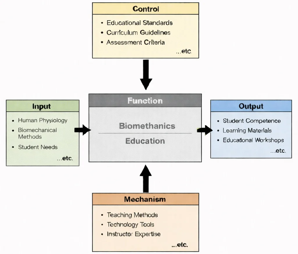
IDEF0 view of Biomechanics Education: physiology and biomechanical methods guided by standards and assessment, enabled by teaching and tools, producing student competence and learning resources.

Biomechanics lies at the intersection of mechanics and biology, focusing on the structure, function, and motion of biological systems. As a key branch of Biomedical Engineering, it applies principles from classical mechanics to analyze how forces affect the human body, prosthetic devices, and tissue systems. Foundational understanding from Bioinformatics and Biomaterials supports research into how genetic factors and engineered materials interact with biomechanical environments.

The study of dynamic body motion requires inputs from Biomedical Signal Processing to monitor muscle activation, and from Medical Imaging to visualize joints, bones, and tissue deformations. Biomechanics also plays a crucial role in the design and optimization of cardiovascular devices within Cardiovascular Engineering, and in refining neural interface systems in Neural Engineering. Moreover, biomechanics enables the practical testing and deployment of innovations within Clinical Engineering.

Drug delivery and biomechanical feedback mechanisms overlap in the realm of Pharmaceutical Engineering, particularly when material deformation affects dosage timing. In Rehabilitation Engineering, biomechanics is central to designing adaptive braces, orthotic supports, and exoskeletons. Similarly, the creation of functional tissues in Tissue Engineering and Regenerative Medicine depends on understanding how mechanical cues influence cellular behavior.

The scope of biomechanics extends into allied fields such as Chemical Engineering, where engineered reactions in living tissues are guided by principles also seen in Biochemical Engineering and Chemical Catalysis and Reaction Engineering. Mechanical testing of biomaterials benefits from knowledge in Chemical Materials Engineering and manufacturing insights from Chemical Process Engineering. Simulations using tools from Computational Chemical Engineering help model tissue deformation and fluid interaction.

Applications extend further into areas like Food and Beverage Engineering, where biomechanical properties influence food texture and processing. Miniaturized sensors and smart responses developed in Nanotechnology in Chemical Engineering enhance performance monitoring of biomechanical systems. The synergy with Polymer and Plastics Engineering is evident in the development of stretchable and responsive materials used in body-mounted devices and flexible prosthetics.

Insights from structural engineering disciplines such as Civil Engineering help analyze load-bearing capacities in artificial joints and bone replacements. Project coordination lessons from construction management can also aid the design of clinical testing frameworks for biomechanical equipment. Additionally, the resilience frameworks used in Earthquake and Disaster Engineering mirror the robustness required in biomechanical implants exposed to dynamic and repetitive stress conditions.

Futuristic biomechanics scene showing a translucent running human with highlighted muscles and joints, surrounded by skeletal diagrams, force vectors, and orthopedic implants on a digital blue interface.

Biomechanics uses physics and anatomy to understand how the body moves, absorbs forces, and avoids injury. This illustration portrays biomechanics as the science of motion and load in the human body. At the center, a semi-transparent runner is rendered with visible muscle fibers and emphasized joints, suggesting analysis of gait, posture, and joint mechanics. Around the figure, skeletal reference panels and data-style overlays indicate measurement and modelling—such as force distribution, impact, and alignment. On the left, orthopedic components such as hip and knee implants connect the study of movement to clinical applications, including rehabilitation and prosthetic or implant design. Overall, the image communicates how biomechanics combines anatomy, engineering, and data to improve performance, safety, and medical outcomes.

Biomedical Engineering – Knowledge Map

Explore how Biomechanics connects across the broader Biomedical Engineering curriculum roadmap. This unified cluster map illustrates the strategic relationship between musculoskeletal kinetics, tissue mechanics, joint implants, and rehabilitation systems:

Biomedical Engineering – Overview

Situates biomechanical analysis within the wider effort to understand and support human function through engineering principles and integrative technological design.

Biomechanics (Current Module)

Examines how internal and external forces, kinematic movement, and material properties govern movement, structural stability, and injury mechanisms across biological systems.

Biomaterials

Determines how synthetic and natural materials respond mechanically to physiological stresses and strains when integrated into bone, joint, and soft tissue structures.

Tissue Engineering & Regenerative Medicine

Recreates specific biomechanical microenvironments and mechanical strain cues that guide cellular differentiation and restore fully functional tissue behavior.

Cardiovascular Engineering

Studies hemodynamics, fluid velocity vectors, and wall shear stress dynamics that govern blood circulation, vascular elasticity, and heart valve mechanics.

Neural Engineering

Links biomechanical movement with motor control pathways, examining how neural impulses translate into mechanical forces and coordinated muscle activation.

Medical Imaging

Captures volumetric 3D structural geometries and dynamic motion tracking data to visualize and quantify biomechanical loading in living subjects.

Biomedical Signal Processing

Processes electromyographic (EMG) muscle activity and sensor telemetry data to extract quantitative metrics on muscle fatigue and movement efficiency.

Bioinformatics

Provides mechanobiological and genomic insights that explain how cellular structures sense, transduce, and adapt to long-term mechanical loading at the molecular level.

Pharmaceutical Engineering

Considers how therapeutic compounds and targeted drug delivery systems influence tissue viscoelasticity, healing processes, and mechanical stress resilience.

Rehabilitation Engineering

Applies biomechanical principles to design assistive exoskeletons, custom orthotics, and adaptive mobility systems that restore independent movement.

Clinical Engineering

Ensures that motion capture systems, force plates, and biomechanical clinical diagnostic hardware operate safely, accurately, and in compliance with healthcare standards.

Core Concepts in Biomechanics

Kinematics

Definition: The study of motion without considering the forces that cause it.
Focus Areas:
- Displacement, velocity, and acceleration of body segments.
- Analysis of gait, joint angles, and body movements.
Applications:
- Evaluating running and walking patterns to improve athletic performance or rehabilitate injuries.

Kinetics

Definition: The study of forces and torques that cause motion.
Focus Areas:
- Ground reaction forces, joint forces, and muscle forces.
- Interaction between internal forces such as muscle contractions and external forces such as gravity and friction.
Applications:
- Designing orthopedic implants to withstand physical loads.
- Analyzing the impact of sports movements on joints to prevent injuries.

Tissue Mechanics

Definition: The study of the mechanical behavior of biological tissues such as bones, muscles, tendons, and ligaments.
Focus Areas:
- Stress-strain relationships of biological tissues.
- Material properties such as elasticity, plasticity, and viscoelasticity.
Applications:
- Designing more durable and biocompatible prosthetics and implants.

Fluid Biomechanics

Definition: Analysis of fluid flow within biological systems.
Focus Areas:
- Blood flow in arteries and veins.
- Airflow in the respiratory system.
Applications:
- Understanding cardiovascular diseases.
- Designing artificial heart valves and vascular grafts.

Neuromuscular Biomechanics

Definition: The interaction between the nervous system and the musculoskeletal system to produce movement.
Focus Areas:
- Muscle activation patterns.
- Coordination of movement.
Applications:
- Rehabilitation robotics.
- Exoskeleton design for mobility support.

Applications of Biomechanics

Prosthetics and Orthotics

Prosthetics:
- Designing artificial limbs that mimic natural movement.
- Incorporating lightweight and durable materials to improve comfort and function.
- Using robotics and AI to enhance control and mobility in prosthetic limbs.
Orthotics:
- Creating supportive devices to correct or accommodate musculoskeletal deformities.
- Custom orthotic insoles to improve gait and reduce pain.

Orthopedics

Implant Design:
- Developing joint replacements, such as hip, knee, and shoulder implants, that withstand biomechanical loads.
- Creating spinal implants and fixation devices.
Bone and Joint Health:
- Studying the mechanical behavior of bones to prevent fractures and degenerative diseases.
- Optimizing surgical procedures such as ACL reconstruction using biomechanical data.

Sports Biomechanics

Performance Enhancement:
- Analyzing athletes’ movements to improve technique and performance.
- Designing sport-specific equipment, such as running shoes or golf clubs, for better efficiency.
Injury Prevention:
- Identifying harmful movement patterns to reduce the risk of injury.
- Developing protective gear to minimize impact forces.

Rehabilitation Engineering

Assistive Devices:
- Designing exoskeletons and robotic devices to restore mobility in patients with neurological injuries.
- Developing smart wheelchairs and mobility aids.
Therapy Optimization:
- Using motion analysis to guide physical therapy.
- Customizing rehabilitation programs based on biomechanical feedback.

Ergonomics and Workplace Safety

Workplace Design:
- Optimizing workstation design to reduce repetitive strain injuries.
- Designing tools and equipment to align with human biomechanics.
Manual Handling:
- Developing lifting techniques and supportive gear to prevent musculoskeletal injuries.

Biomedical Device Development

Wearable Technology:
- Designing wearable sensors to monitor joint movement, posture, and muscle activity.
Implantable Devices:
- Creating bioengineered implants that adapt to mechanical stress in the body.

Technologies in Biomechanics

Motion Capture Systems

Function: Tracks and analyzes body movement in 3D.
Applications: Sports performance analysis, rehabilitation, and gait analysis.

Force Plates and Pressure Sensors

Function: Measures ground reaction forces and pressure distribution.
Applications: Assessing balance, gait, and jump dynamics; studying injury risks in athletes.

Finite Element Analysis (FEA)

Function: Simulates how biological structures respond to external forces.
Applications: Designing orthopedic implants and prosthetics; evaluating mechanical strength of bones and tissues.

Electromyography (EMG)

Function: Measures electrical activity in muscles.
Applications: Assessing muscle activation patterns; diagnosing neuromuscular disorders.

Computational Modeling and Simulation

Function: Creates digital models of biological systems for analysis.
Applications: Simulating joint mechanics under different movement scenarios; predicting performance of medical devices.

Contemporary AI-Era Computational Paradigms in Biomechanics

Modern biomechanical analysis has expanded beyond classical rigid-body link segment models and empirical inverse dynamics into high-fidelity neural surrogate models and physics-informed computational simulations:

1. Physics-Informed Neural Networks (PINNs) for Viscoelastic Soft Tissue Modeling: Ligaments, tendons, and cartilage exhibit non-linear viscoelasticity, exhibiting creep and strain-rate dependency governed by fractional constitutive equations. PINNs incorporate continuum mechanics equilibrium ($\nabla \cdot \boldsymbol{\sigma} + \mathbf{f} = \rho \ddot{\mathbf{u}}$) directly into training loss functions, enabling instantaneous inverse estimation of internal ligament stresses from non-invasive surface strain measurements.

Numerical Illustration: Single-Leg Stance Hip Abductor Force & Joint Reaction Equilibrium

During single-leg stance, an individual of body mass $m = 70.0 \text{ kg}$ supports their entire body weight on one limb. The effective mass of the body excluding the stance leg is $m_{\text{trunk}} = 56.0 \text{ kg}$, acting at a horizontal moment arm $d_1 = 10.0 \text{ cm}$ ($0.10 \text{ m}$) medial to the hip joint rotation center. The gluteus medius abductor muscle complex inserts laterally with an effective moment arm $d_2 = 5.0 \text{ cm}$ ($0.05 \text{ m}$), oriented at an angle $\theta = 70.0^\circ$ relative to the horizontal. Calculate the required abductor muscle force $F_M$ for static moment equilibrium, and evaluate the resultant hip Joint Reaction Force ($\text{JRF}$) magnitude:

$$\sum M_{\text{hip}} = 0 \Rightarrow W_{\text{trunk}} \cdot d_1 - F_M \cdot d_2 = 0$$

Step 1: Compute trunk gravitational body weight force $W_{\text{trunk}}$ ($g = 9.81 \text{ m/s}^2$):

$$W_{\text{trunk}} = 56.0 \text{ kg} \times 9.81 \text{ m/s}^2 = \mathbf{549.36 \text{ N}}$$

Step 2: Solve for abductor muscle tensile force $F_M$ about the hip fulcrum:

$$F_M = \frac{W_{\text{trunk}} \cdot d_1}{d_2} = \frac{549.36 \text{ N} \times 0.10 \text{ m}}{0.05 \text{ m}} = \mathbf{1,098.72 \text{ N}}$$

Step 3: Resolve forces along horizontal ($x$) and vertical ($y$) axes to determine $\text{JRF}$:

$$\sum F_x = 0 \Rightarrow JRF_x = F_M \cos(70^\circ) = 1,098.72 \times 0.34202 = \mathbf{375.78 \text{ N}}$$ $$\sum F_y = 0 \Rightarrow JRF_y = W_{\text{trunk}} + F_M \sin(70^\circ) = 549.36 + (1,098.72 \times 0.93969) = 549.36 + 1,032.46 = \mathbf{1,581.82 \text{ N}}$$ $$JRF = \sqrt{(JRF_x)^2 + (JRF_y)^2} = \sqrt{(375.78)^2 + (1,581.82)^2} = \sqrt{141,210.6 + 2,502,154.5} = \mathbf{1,625.96 \text{ N}}$$

Biomechanical Interpretation: Total compressive joint reaction force on the femoral head reaches $1,626.0 \text{ N}$ ($\approx 2.37 \times$ total body weight) during static single-leg balance. This dramatic mechanical amplification highlights why maintaining abductor muscle strength is vital for minimizing osteoarthritis wear in prosthetic hip replacements.

2. Deep Learning Markerless Kinematics & Pose Estimation: Classical optical motion capture requires physical retro-reflective skin markers that suffer from soft-tissue motion artifacts. Deep neural networks (e.g., spatio-temporal graph convolutional networks) process multi-view high-speed video feeds directly, estimating 3D anatomical joint centers and skeletal kinematics with sub-millimeter precision.

3. Multiscale Musculoskeletal Digital Twins: Patient-specific digital twins combine automated segmentation of clinical MRI/CT scans with rigid-body neuromuscular forward dynamics, running in-silico clinical trials to evaluate implant contact pressures before surgical intervention.

Engineering Trade-offs in Biomechanics

Engineering orthotic, prosthetic, and implantable biomechanical systems requires balancing structural stiffness, biological remodeling, wear durability, and energetic cost:

Biomechanical Design Trade-off	Primary Engineering Benefit	Systemic Penalty / Risk	Quantitative Design Metric
Titanium Alloy (Ti-6Al-4V) vs. Cobalt-Chromium (CoCr) Femoral Stems	Lower Young's modulus ($E \approx 110 \text{ GPa}$) closer to cortical bone ($E \approx 18 \text{ GPa}$), reducing stress shielding bone loss.	Lower abrasive wear resistance compared to CoCr when functioning as direct articulating bearing surfaces.	Elastic Modulus Match: Ti-6Al-4V ($110 \text{ GPa}$); CoCr ($210\text{--}240 \text{ GPa}$).
Rigid Carbon-Fiber AFO vs. Articulated Dynamic Ankle Orthosis	Maximizes energy storage and return during push-off; maximum coronal and sagittal plane stability.	Eliminates normal ankle joint range of motion, inducing compensatory knee hyperextension during terminal stance.	Stiffness Coefficient: Rigid AFO ($K_{\text{rot}} \ge 3.0 \text{ N}\cdot\text{m/deg}$).
Porous Trabecular Ingrowth Surfaces vs. PMMA Bone Cement Fixation	Biological osseointegration creates permanent living bone-implant interface, preventing late cement debonding.	Requires strict initial micromotion limits ($< 50 \text{ \mu m}$) during immediate post-operative period to prevent fibrous tissue encapsulation.	Interfacial Shear Strength: Biological Osseointegration ($\ge 15 \text{ MPa}$).
Powered Robotic Knee-Ankle Prosthesis vs. Passive Elastic Blade	Actively injects positive mechanical work during toe-off, normalizing metabolic oxygen consumption during uphill gait.	Substantial mass penalty ($>4.0 \text{ kg}$), limited battery life ($8\text{--}12 \text{ hours}$), and acoustic actuator noise.	Metabolic Cost of Transport: Powered Prosthesis saves $15\text{--}25\%$ net metabolic energy.

Quantitative Trade-off Illustration: Stress Shielding in Cortical Bone Implants

According to Wolff's Law of bone remodeling, bone tissue resorbs in regions where functional mechanical stress drops below homeostatic remodeling thresholds. In a composite femoral structure composed of cortical bone (cross-sectional area $A_b = 350.0 \text{ mm}^2$, Young's modulus $E_b = 18.0 \text{ GPa}$) and an intramedullary stem ($A_s = 150.0 \text{ mm}^2$), calculate the fraction of an axial compressive gait load $P = 2,500.0 \text{ N}$ transferred through the stem if the stem is manufactured from (a) Titanium Alloy ($E_s = 110.0 \text{ GPa}$) versus (b) Stainless Steel ($E_s = 200.0 \text{ GPa}$):

$$\text{Axial Rigidity} = (EA)_{\text{total}} = E_b A_b + E_s A_s$$ $$\text{Load Fraction Carried by Stem} = \frac{E_s A_s}{(EA)_{\text{total}}} = \frac{E_s A_s}{E_b A_b + E_s A_s}$$

Step 1: Compute bone axial stiffness $E_b A_b$:

$$E_b A_b = 18.0 \text{ GPa} \times 350.0 \text{ mm}^2 = \mathbf{6,300.0 \text{ kN}}$$

Step 2: Case A - Titanium Stem ($E_s = 110.0 \text{ GPa}$):

$$E_{s,\text{Ti}} A_s = 110.0 \text{ GPa} \times 150.0 \text{ mm}^2 = 16,500.0 \text{ kN}$$ $$\text{Fraction}_{\text{Ti}} = \frac{16,500.0}{6,300.0 + 16,500.0} = \frac{16,500.0}{22,800.0} = \mathbf{72.37\%} \quad (\text{Bone carries } 27.63\%)$$

Step 3: Case B - Stainless Steel Stem ($E_s = 200.0 \text{ GPa}$):

$$E_{s,\text{Steel}} A_s = 200.0 \text{ GPa} \times 150.0 \text{ mm}^2 = 30,000.0 \text{ kN}$$ $$\text{Fraction}_{\text{Steel}} = \frac{30,000.0}{6,300.0 + 30,000.0} = \frac{30,000.0}{36,300.0} = \mathbf{82.64\%} \quad (\text{Bone carries } 17.36\%)$$

Design Assessment: The stiffer stainless steel implant absorbs 82.6% of the gait load, leaving the host cortical bone under-stimulated (carrying only 17.4% of axial force). This triggers extensive proximal osteopenia and implant loosening over decadal timeframes, demonstrating why lower-modulus porous titanium alloys are preferred.

Interactive Biomechanical Gait & Joint Force Simulator

Utilize this interactive engineering simulator to analyze the joint reaction forces (JRF), muscle moment arms, and ground reaction forces (GRF) during locomotion. Adjust body mass, cadence, and knee flexion angle to observe real-time biomechanical load changes during stance phase.

Subject Body Mass (kg): 70

Knee Flexion Angle (θ): 25°

Locomotion Activity:

Ground Reaction Force (GRF) Stance Curve

Joint Reaction Force (Patellofemoral JRF)

Calculating dynamic biomechanical parameters...

Interactive runtime environment: https://prep4uni.online/stem/physical-technologies/biomedical-engineering/biomechanics/

Challenges in Biomechanics

Biomechanics, as a discipline at the intersection of biology, physics, and engineering, plays a vital role in understanding human movement, designing prosthetics, optimizing surgical interventions, and simulating biological function. However, this rapidly evolving field faces several formidable challenges. These range from biological variability to technological limitations and ethical complexities. Addressing these issues is crucial for advancing both research and clinical applications in biomechanics.

Complexity of Biological Systems

Inherent Variability: Each human body differs significantly in size, muscle strength, bone density, and joint mobility, making it difficult to create standardized biomechanical models. Age, sex, ethnicity, and lifestyle factors further complicate generalization.
Tissue Behavior: Biological tissues are anisotropic, viscoelastic, and non-linear in their mechanical behavior. This makes modeling them far more difficult than simple engineering materials.
Dynamic Interactions: The interplay between muscles, bones, tendons, and neural control systems varies continuously with time and activity, introducing additional layers of complexity.

Integration of Multidisciplinary Knowledge

Cross-Disciplinary Expertise: Effective biomechanical analysis requires knowledge in anatomy, physiology, mechanical engineering, materials science, computer science, and clinical medicine. The breadth of knowledge required creates a high barrier to entry for researchers and practitioners.
Communication Barriers: Different disciplines often use different terminologies, data standards, and software tools, making collaborative work challenging.
Educational Gaps: Most university programs do not fully integrate this interdisciplinary knowledge into a single curriculum, resulting in professionals with gaps in one or more key domains.

Data Accuracy and Validation

Measurement Challenges: Accurate real-time data on internal body mechanics is difficult to acquire non-invasively. Techniques like motion capture, force plates, and imaging have limitations in resolution and fidelity.
Model Validation: Validating simulations against in vivo conditions is difficult due to ethical constraints and technological limits in tracking internal structures like ligaments or cartilage under load.
Environmental Variation: Real-world conditions such as uneven terrain, fatigue, or disease progression introduce variability that cannot be fully replicated in laboratory settings.

Ethical Considerations

Human Subject Research: Biomechanical testing on living subjects must comply with strict ethical standards. The need to avoid harm limits invasive measurements and testing, especially for vulnerable populations such as children or the elderly.
Animal Testing: While often necessary, animal models do not always accurately reflect human biomechanics, and their use raises ethical concerns in research communities.
AI and Bias: The growing use of AI in biomechanical prediction, such as gait analysis or injury risk estimation, raises concerns about algorithmic bias and equity in treatment outcomes.

Customization of Solutions

Personalization Needs: Effective prosthetic and orthotic solutions must be custom-designed for individual anatomy and activity level, requiring detailed imaging and patient data.
Manufacturing Limits: Additive manufacturing has revolutionized customization, but still faces issues with material biocompatibility, mechanical integrity, and regulatory approval.
Cost and Accessibility: Custom devices are expensive and often unavailable in resource-limited settings, raising concerns about global health equity.

Computational Limitations and Simulation Complexity

High Computational Demand: Accurate simulations, particularly those involving finite element models of human joints or muscles, are computationally expensive and time-consuming.
Real-Time Analysis: For applications in wearable technologies or surgical robotics, biomechanical models must compute in real time, a capability still under development.
Data Fusion: Integrating data from sensors such as EMG, IMU, and ultrasound into a unified model without loss of accuracy or latency is an ongoing challenge.

Translational Gaps Between Research and Clinical Practice

Limited Adoption: Many advanced biomechanical tools remain underused in clinical settings due to complexity, lack of training, or regulatory barriers.
Workflow Integration: Integrating biomechanical data into electronic health records and decision-support systems is still in its infancy.
Outcome Measurement: There is often a lack of standardized metrics to evaluate the effectiveness of biomechanical interventions in real-world healthcare environments.

To learn more about emerging solutions and tools in biomechanics, explore the NIH open-access biomechanics research overview and The Journal of Biomechanics for recent peer-reviewed publications.

Conclusion

While the challenges in biomechanics are multifaceted and deeply intertwined with the complexities of the human body, they also present immense opportunities for innovation. As data acquisition improves, computational power expands, and interdisciplinary collaboration strengthens, these obstacles can be systematically overcome. Addressing these hurdles will not only accelerate scientific discovery but also enhance patient-specific care, injury prevention, rehabilitation strategies, and the performance of medical devices for diverse populations around the world.

Future Trends in Biomechanics

Smart Prosthetics and Wearables

Smart prosthetics are evolving beyond basic mechanical functionality to incorporate embedded sensors, artificial intelligence, and responsive control systems. These technologies enable real-time feedback and adjustments, allowing prosthetic limbs to respond dynamically to user intentions and environmental changes. Wearable biomechanics devices also track gait, muscle activity, and joint movement, offering data for clinicians to personalize rehabilitation strategies. This trend is driving improvements in both comfort and functionality for individuals with limb loss or motor impairments.

Brain-computer interfaces are also being integrated into advanced prosthetics, enabling users to control limbs through neural signals. Wearables in biomechanics are used to monitor athletes’ performance, prevent injuries in sports science, and support occupational ergonomics.

3D Printing of Customized Implants

Additive manufacturing, or 3D printing, is transforming the production of orthopedic implants, dental fixtures, and assistive devices by enabling highly customized designs that fit individual anatomical structures. Engineers can now print implants with porous structures that encourage bone ingrowth, enhancing integration with the patient’s body.

3D printing also allows rapid prototyping of biomechanics tools and the production of lightweight, durable devices using materials such as titanium, polymers, and composite biomaterials. Surgeons can use 3D-printed anatomical models to plan complex procedures and improve surgical accuracy.

Bioengineered Tissues and Organs

Researchers are developing bioengineered tissues that replicate the biomechanical properties of natural ligaments, tendons, and cartilage. These engineered tissues can be used for reconstructive surgery, sports injury recovery, and organ transplantation. Advances in biomechanics inform the mechanical conditioning of these tissues during cultivation, mimicking physiological stresses to support functional performance.

Scaffold-based regeneration, bioprinting of vascular networks, and stem cell integration are all areas of active development. These approaches aim to address limitations in donor availability and rejection in organ transplantation, while also supporting personalized regenerative medicine.

Virtual Reality and Augmented Reality in Biomechanical Training

Virtual reality and augmented reality are being used in physical rehabilitation, surgical training, and movement re-education. These immersive technologies provide real-time biomechanical feedback and simulate realistic environments to engage patients more effectively during therapy. VR-enhanced gait training is used for stroke recovery, while AR-assisted procedures help surgeons visualize internal anatomical structures with overlaid biomechanical data.

Biomechanics-informed simulations also help researchers test implant behavior and movement patterns in a risk-free digital environment before translating them into clinical practice, reducing trial-and-error and enhancing patient safety.

Machine Learning and Big Data Analytics

The integration of machine learning into biomechanics enables the analysis of massive datasets generated by motion capture, force plates, electromyography, and imaging tools. These insights are critical for recognizing abnormal movement patterns, predicting injury risks, and improving the design of assistive devices and orthopedic interventions.

Predictive analytics is being used to tailor rehabilitation protocols, while real-time monitoring of post-operative recovery can help clinicians intervene proactively. AI models can also help researchers understand subtle biomechanical interactions within musculoskeletal systems that were previously difficult to capture through conventional analysis.

Digital Twins and Biomechanical Simulation

Digital twins—virtual replicas of anatomical systems—are being developed for biomechanical simulations of joints, muscles, and soft tissues. These models enable researchers to test implant mechanics, simulate surgical outcomes, and evaluate physical therapy techniques with high accuracy. Combined with real-time patient data, digital twins support personalized treatment planning and performance assessment.

Advanced simulations also aid in the design of smart textiles and responsive orthotics that adapt to biomechanical feedback, enhancing comfort and effectiveness.

Exoskeletons and Assistive Robotics

Exoskeletons are wearable biomechanical systems that support or enhance human movement. Originally developed for rehabilitation and military applications, they are now being explored in industrial settings to reduce musculoskeletal strain and fatigue among workers. Clinical-grade robotic exosuits aid individuals with spinal cord injuries, stroke, or muscular dystrophy to regain mobility.

Future models will incorporate AI, machine learning, and real-time EMG analysis to create more intuitive, adaptive control systems. The long-term vision includes full lower-limb replacement systems for patients with paralysis or degenerative disorders.

Neurobiomechanics and Brain-Body Interfaces

Neurobiomechanics is an emerging field that studies how the nervous system and biomechanical structures interact during movement. By combining neuroscience with motion science, researchers aim to develop advanced prosthetics, rehabilitation tools, and neural implants. Brain-machine interfaces and spinal stimulation devices show promise in restoring motor function and controlling prosthetic devices.

These developments offer hope for individuals with neurological conditions such as ALS, cerebral palsy, and spinal cord injury, enabling partial or even full restoration of movement with minimally invasive intervention.

Biomechanics in Space Exploration and Aging

Space agencies are leveraging biomechanics to understand the effects of microgravity on musculoskeletal health. Research on astronauts’ bone and muscle degradation informs countermeasure designs, such as resistive exercise devices and nutrient delivery systems. Similar principles are applied to geriatrics to prevent falls, manage osteoporosis, and improve mobility in aging populations.

These insights contribute to the development of assistive devices, adaptive footwear, and mobility aids that help older adults maintain independence and reduce injury risk.

Sustainable and Bioinspired Materials

Future biomechanics devices will increasingly incorporate biodegradable, sustainable, and bioinspired materials that mimic the flexibility and strength of biological tissues. Examples include spider silk-inspired fibers and self-healing polymers that respond to stress or damage. These materials improve the longevity and ecological footprint of biomedical devices and wearables.

Such sustainable solutions are aligned with global goals for environmental responsibility and health equity, especially in resource-constrained healthcare systems.

Why Study Biomechanics

Understanding Human Motion and Forces: Biomechanics studies how forces act on the human body during movement. Students learn to analyze walking, running, lifting, and joint function. This knowledge supports rehabilitation, sports science, and ergonomic design.

Applications in Prosthetics and Orthopedics: Students explore how biomechanical principles guide the design of prosthetic limbs and orthopedic implants. They evaluate how devices interact with muscle and bone. This ensures comfort, function, and long-term performance.

Modeling and Simulation Tools: The field relies on computer models to simulate body mechanics and predict outcomes. Students learn to use software to analyze stresses and movements. These tools enhance research and clinical decision-making.

Injury Prevention and Rehabilitation: Biomechanics helps identify causes of injury and guide recovery strategies. Students apply motion analysis and force measurement to improve therapy. This contributes to safer environments and effective treatments.

Interdisciplinary Research and Impact: The field integrates physiology, engineering, and physics. Students can pursue careers in healthcare, research, and sports performance. Biomechanics plays a key role in enhancing human health and function.

Biomechanics: Conclusion

Biomechanics stands at the intersection of biology, physics, engineering, and medicine, offering a powerful framework for analyzing and enhancing how living systems move and function. This multidisciplinary field has evolved into a cornerstone of modern healthcare, athletics, rehabilitation, and even aerospace and robotics. Through the application of mechanical principles to biological tissues, biomechanics enables researchers, clinicians, and engineers to develop innovative solutions that improve mobility, optimize performance, and extend quality of life across age groups.

Impact on Healthcare and Prosthetics

One of the most transformative contributions of biomechanics is in the realm of medical devices, especially prosthetics and orthopedic implants. By simulating joint movement, tissue loading, and muscle forces, biomechanical models inform the design of prosthetic limbs that closely replicate natural motion. These advancements not only restore mobility to individuals with limb loss but also significantly improve comfort, fit, and usability. Similarly, joint replacements—such as hip and knee implants—benefit from precise biomechanical testing to ensure long-term durability under physiological loads.

Technologies like finite element analysis and motion capture systems allow engineers to simulate patient-specific conditions, leading to better surgical planning and customized implants. In spinal surgery, biomechanics has enhanced the development of vertebral fixation systems and intervertebral discs that align with the spine’s complex kinematics.

Revolutionizing Rehabilitation and Physical Therapy

Biomechanics has become a vital tool in rehabilitation engineering, supporting the recovery of patients following injury, surgery, or neurological disorders. Gait analysis systems track how individuals walk or run, enabling therapists to detect abnormalities, measure progress, and tailor treatment plans. For stroke patients, wearable motion sensors combined with biomechanical algorithms help guide motor retraining and monitor functional improvement.

Orthotic devices, such as ankle-foot orthoses or dynamic splints, are now designed based on individual biomechanical needs, improving alignment, reducing pain, and supporting efficient movement patterns. Biomechanics also supports remote rehabilitation and telehealth by integrating data from wearable sensors into mobile applications and cloud-based platforms.

Performance Optimization in Sports and Exercise Science

Athletes and coaches rely on biomechanics to refine movement techniques, prevent injuries, and maximize physical output. High-speed cameras, force plates, and electromyography allow for detailed assessments of muscle activity, joint angles, and force application. These insights are used to optimize running strides, improve pitching mechanics, or enhance cycling posture.

Biomechanics also aids in return-to-play protocols by providing objective criteria for recovery. For example, an athlete recovering from a serious knee injury may undergo 3D motion analysis to ensure movement patterns have recovered before returning to competition.

Applications in Ergonomics and Workplace Safety

In occupational health and ergonomics, biomechanics plays a key role in reducing workplace injuries and enhancing productivity. By analyzing how workers lift, carry, or perform repetitive motions, experts can redesign tools, workstations, and workflows to reduce strain and musculoskeletal disorders. Ergonomic chairs, standing desks, and wearable supports are often developed with biomechanical data to improve safety and comfort.

Biomechanics is also central to developing exoskeletons that assist with lifting heavy loads or supporting fatigued muscles, increasingly used in industrial and military contexts.

Driving Innovation in Robotics and Human-Machine Interfaces

The principles of biomechanics are essential in the design of humanoid robots, assistive robotics, and brain-computer interfaces. By mimicking the structure and function of the musculoskeletal system, engineers are developing robotic systems capable of navigating human environments with agility and balance. In assistive technology, biomechanical modeling ensures robotic limbs or exosuits move in harmony with the user’s body, reducing fatigue and increasing functionality.

Brain-computer interfaces combined with biomechanical control loops offer the possibility of restoring mobility for individuals with paralysis or neurodegenerative diseases. Such innovations are shaping the future of mobility and autonomy for many patients.

Contributions to Aging and Fall Prevention

As populations age, biomechanics becomes increasingly relevant in fall prevention, fracture risk assessment, and mobility support. Researchers develop biomechanical models to understand balance impairments and develop interventions such as balance training programs, anti-slip footwear, and assistive walkers. Wearable devices track motion patterns to alert users or caregivers about potential risks in real time.

In the context of osteoporosis, biomechanics is used to analyze bone strength and predict fracture sites, influencing both treatment planning and lifestyle recommendations.

Educational and Research Significance

Biomechanics has also become a cornerstone of research and higher education in biomedical engineering, kinesiology, physical therapy, and mechanical engineering. Students learn to use simulation software, conduct experimental motion analysis, and integrate biological knowledge into mechanical systems. This foundation prepares the next generation of innovators who will continue advancing healthcare, sports, and human performance technologies.

The research community is constantly expanding the frontier of biomechanics by exploring cellular mechanobiology, organ-level deformation, and molecular force transmission, providing deeper insight into how mechanical forces influence biological function at all scales.

Environmental and Global Health Applications

Beyond clinical and performance settings, biomechanics contributes to global health initiatives. In resource-limited environments, biomechanically optimized crutches, prosthetics, and orthopedic braces are being developed with cost-effective materials. These solutions provide support to individuals affected by conflict, disease, or natural disasters. Organizations such as the World Health Organization emphasize the importance of assistive technologies, including those developed through biomechanical research, for improving accessibility and independence.

Future Outlook: Boundless Potential

As technologies like artificial intelligence, virtual reality, 3D printing, and bioinspired design continue to mature, biomechanics will further integrate into daily life. Smart prosthetics that respond to thought, digital twins of human joints for predictive modeling, and biodegradable implants that adapt to body dynamics represent just a fraction of what lies ahead. The synergy between biomechanics and these emerging tools will lead to more personalized, effective, and sustainable health interventions.

The future of biomechanics holds the promise of transforming not only how injuries are treated or performance is optimized, but also how we understand the human experience through the lens of movement and mechanical interaction with the world.

References

Frequently Asked Questions on Biomechanics

Why is biomechanics so central to modern biomedical engineering?

Biomechanics sits at the meeting point of physics, engineering, and anatomy. By treating the body as a system of forces, motions, and materials, it helps us understand why joints wear out, how injuries occur, and what makes movement efficient or painful. This knowledge is essential for designing implants, prosthetics, rehabilitation devices, and surgical techniques that work with the body instead of against it.

Is biomechanics only about sports and elite athletes?

Elite sport provides striking examples, but biomechanics is just as relevant to everyday activities such as walking, lifting, or climbing stairs. The same principles apply when designing safer workplaces, fall-prevention strategies for older adults, or better wheelchairs and walking aids. In that sense, biomechanics is about movement for everyone, not only for top performers.

How mathematical is biomechanics as a subject?

Biomechanics uses the language of mechanics: forces, moments, equilibrium, stress, and strain. Students do not have to be mathematicians, but comfort with basic algebra, vectors, and Newton’s laws is helpful. At university level, the subject gradually introduces more formal modelling, such as differential equations or finite element analysis, but always with the goal of explaining real movement and real devices.

What is the difference between musculoskeletal biomechanics and biofluid mechanics?

Musculoskeletal biomechanics focuses on bones, muscles, tendons, ligaments, and joints, asking how they generate and transmit forces during movement. Biofluid mechanics examines the flow of biological fluids such as blood, cerebrospinal fluid, or air in the lungs. Both areas rely on the same physical principles, but one treats the body as a system of levers and supports, while the other treats it as a system of channels and flows.

How does biomechanics influence the design of prosthetic limbs?

In prosthetic design, biomechanics provides target values for joint angles, step lengths, and ground reaction forces that resemble natural gait. Engineers use these data to choose appropriate materials, align components, and design control systems so that the prosthesis feels stable, efficient, and comfortable. Biomechanics also helps evaluate new designs by comparing how closely they reproduce healthy movement patterns.

Where does biomechanics connect with rehabilitation and clinical practice?

Clinicians use biomechanical measurements—such as gait analysis, pressure mapping, or motion capture—to understand why a patient moves in a particular way. Engineers then translate these findings into supports, exercises, or devices that reduce harmful loading and strengthen useful movement patterns. In this partnership, biomechanics acts as the common framework that links clinical observations to engineering solutions.

What should a student look out for when first studying biomechanics?

It helps to constantly connect equations back to simple questions: Where is this force coming from? Which structure is carrying it? How might this change if the person were older, injured, or running instead of walking? Keeping that link between mathematics and the moving body makes biomechanics both more memorable and more useful for future study and professional work.

Interactive Concept Review Exercises

Toggle each box below to reveal detailed answers and conceptual breakdowns.

Review Question 1: How does the analysis of gait biomechanics contribute to the design of lower-limb prosthetics?

Explanation: Gait biomechanics quantifies kinematics (joint trajectories) and kinetics (ground reaction forces). By matching these parameters, engineers can select energy-storing materials and active actuators that replicate natural ankle/knee mechanics during stance and swing phases.

Review Question 2: Why are biological soft tissues characterized as viscoelastic?

Explanation: Biological soft tissues (ligaments, tendons, cartilage) exhibit both viscous fluid-like and elastic solid-like properties. Their stress-strain response is rate-dependent, demonstrating phenomena such as creep, stress relaxation, and hysteresis under cyclic loading.

Review Question 3: How does finite element analysis (FEA) assist in orthopedic implant design?

Explanation: FEA discretizes complex anatomical bone geometries into finite meshes, solving stress distributions under physiological loads to optimize implant shape and minimize stress shielding prior to clinical fabrication.

End-of-Page Comprehensive Practice Module

Section 1: Foundational Review Questions

1. What is biomechanics, and what kinds of questions does it try to answer?

Answer: Biomechanics is the study of how forces and motions act on living systems. It investigates questions such as how much load passes through joints during gait, how blood flow shear stresses impact arterial walls, and how mechanical forces regulate cellular gene expression.

2. What are the main subfields of biomechanics commonly discussed in biomedical engineering?

Answer: Main subfields include musculoskeletal biomechanics (bones, muscles, joints), cardiovascular biomechanics (blood flow, heart valves), cellular biomechanics (mechanotransduction, cell stiffness), and biofluid mechanics (fluid dynamics in respiratory/vascular channels).

3. What does musculoskeletal biomechanics investigate, and why is it important for device design?

Answer: It investigates how bones, joints, muscles, tendons, and ligaments share loads and generate movement. Quantitative force and torque data allow engineers to design implants, orthoses, and prostheses that restore function without inducing mechanical failure.

4. How is cardiovascular biomechanics used in the development of cardiovascular devices?

Answer: It analyzes pressure gradients, velocity fields, and wall shear stresses to design vascular stents, synthetic grafts, and heart valves that prevent hemolysis, recirculation stagnation, and thrombus formation.

5. What is cellular biomechanics, and how does it support areas like tissue engineering and cancer research?

Answer: It examines cellular mechanical properties and mechanotransduction. In tissue engineering, mechanical strain guides stem cell differentiation; in cancer research, cell membrane deformation and stiffness dictate metastatic cell migration through extracellular matrices.

6. What does biofluid mechanics study, and which medical technologies rely on it?

Answer: Biofluid mechanics studies biological fluid flow (blood, air, CSF, synovial fluid). Technologies relying on it include ventricular assist devices (VADs), mechanical ventilators, hemodialysis filters, and drug-eluting stents.

7. How do biomechanical principles guide the design of prosthetic limbs and rehabilitation devices?

Answer: They provide baseline physiological kinematic joint trajectories and ground reaction force profiles, enabling robotic exoskeletons and smart prosthetics to deliver matched power assistance during gait cycles.

8. What types of innovations in orthopedic implants have emerged from biomechanical research?

Answer: Innovations include porous trabecular titanium surfaces for osteointegration, flexible composite bone plates that reduce stress shielding, and anatomical ceramic bearing surfaces that minimize wear debris.

9. How do biomechanics and finite element analysis work together in modeling tissues and devices?

Answer: FEA applies mechanical boundary conditions and material constitutive equations to 3D anatomical models, predicting internal stress, strain, and deformation patterns in tissue-device structures under simulated loads.

10. In what ways does biomechanics contribute to rehabilitation, injury prevention, and performance optimization?

Answer: It delivers objective quantitative feedback on movement technique, joint loading, and muscle recruitment patterns, enabling targeted physical therapy, ergonomic workstation adjustments, and safer athletic mechanics.

Section 2: Analytical & Scenario-Based Thought Questions

1. Explain how the lever arm ratio between the Achilles tendon force and ground reaction force affects calf muscle load during human jumping.

Answer: The ankle acts as a second-class or third-class lever depending on foot contact. Because the Achilles tendon moment arm (~5 cm) is significantly shorter than the moment arm of the ground reaction force applied at the forefoot (~15 cm), the gastrocnemius/soleus muscle complex must generate an internal force roughly 3 times greater than the external body weight force to achieve torque equilibrium.

2. Describe the mechanotransduction pathway through which bone osteocytes respond to mechanical loading under Wolff's Law.

Answer: Mechanical loading deforms the calcified bone matrix, driving interstitial fluid flow through the lacunar-canalicular network. Fluid shear stress across osteocyte membranes opens mechanically gated ion channels (e.g., integrins, primary cilia), triggering intracellular calcium influx and signaling pathways (e.g., Wnt/β-catenin) that upregulate osteoblast bone formation and downregulate osteoclast resorption.

3. Why does arterial wall shear stress ($\tau_w$) drop in dilated aneurysmal regions, and what are the biological consequences?

Answer: According to Poiseuille's law ($\tau_w = \frac{4\eta Q}{\pi r^3}$), wall shear stress is inversely proportional to the cube of vessel radius ($r^3$). In an aneurysm, as radius $r$ increases dramatically, wall shear stress drops significantly. Abnormally low shear stress alters endothelial gene expression, promoting localized inflammation, mural thrombus formation, and progressive structural weakening of the vessel wall.

4. Compare the stress-strain behavior of collagen fibers versus elastin fibers in arterial tissue.

Answer: Elastin fibers exhibit high elasticity with a low Young's modulus, extending easily at low physiological pressures to cushion pulsatile blood flow (Windkessel effect). Collagen fibers have a high Young's modulus and remain crimped at low pressures, unravelling and stiffening sharply at higher pressures to prevent excessive arterial distension and structural rupture.

5. How does viscoelastic creep differ from stress relaxation in ligament biomechanics?

Answer: Creep is the time-dependent increase in strain/deformation when a ligament is subjected to a constant tensile load. Stress relaxation is the time-dependent decrease in internal stress observed when a ligament is stretched to and held at a constant deformation.

6. Analyze the biomechanical rationale for placing a cane in the hand opposite to an injured or arthritic hip joint.

Answer: Holding the cane in the contralateral (opposite) hand creates a wide base of support and an upward force with a long moment arm relative to the affected hip center. This counter force provides abductor moment assistance, substantially reducing the required abductor muscle force (gluteus medius) and lowering joint reaction force (JRF) on the arthritic hip by up to 50%.

7. What limits the accuracy of surface electromyography (sEMG) in driving real-time biomechanical inverse dynamics models?

Answer: sEMG suffers from signal cross-talk from adjacent muscles, tissue filtering impedance, motion artifacts, electrode shift, and electromechanical delay (the 30–100 ms lag between electrical membrane depolarization and mechanical force generation), requiring complex filtering and calibration.

Section 3: Quantitative Engineering Calculations

Apply biomechanical equilibrium, tissue constitutive laws, viscoelastic models, and beam torsion formulas to quantitative human motion scenarios. Click each problem below to review full step-by-step calculations.

1. Single-Leg Stance Hip Abductor Muscle Force Calculation

Problem: During single-leg stance, a person of body mass $m = 70.0 \text{ kg}$ supports their body weight. The center of mass of the body excluding the stance leg (mass $m_{\text{trunk}} = 56.0 \text{ kg}$) acts at a distance $d_1 = 10.0 \text{ cm}$ ($0.10 \text{ m}$) from the hip joint center. The hip abductor muscle acts with a moment arm $d_2 = 5.0 \text{ cm}$ ($0.05 \text{ m}$). Calculate the required abductor muscle force ($F_M$) in Newtons for static equilibrium ($g = 9.81 \text{ m/s}^2$).

Answer:

Step 1: Calculate body weight force ($W$) acting on stance hip:
$W = 56.0 \text{ kg} \times 9.81 \text{ m/s}^2 = 549.36 \text{ N}$

Step 2: Set up torque equilibrium around hip joint center ($\sum M = 0$):
$\text{Torque from Body Weight} = W \times d_1 = 549.36 \text{ N} \times 0.10 \text{ m} = 54.936 \text{ N}\cdot\text{m}$
$\text{Torque from Abductor Muscle} = F_M \times d_2 = F_M \times 0.05 \text{ m}$

Step 3: Solve for muscle force ($F_M$):
$F_M \times 0.05 \text{ m} = 54.936 \text{ N}\cdot\text{m} \Rightarrow F_M = \frac{54.936}{0.05} = \mathbf{1,098.72 \text{ N}}$

The required hip abductor muscle force is 1,098.72 N.

2. Articular Cartilage Unconfined Compression & Deformation

Problem: An articular cartilage tissue cylindrical plug (diameter $d = 8.0 \text{ mm}$, length $L_0 = 3.0 \text{ mm}$) is subjected to an unconfined compressive test load $F = 25.0 \text{ N}$. Calculate compressive stress ($\sigma$) in $\text{MPa}$. If the equilibrium compressive modulus $H_A = 0.80 \text{ MPa}$, calculate the total length decrease ($\Delta L$) in $\text{mm}$.

Answer:

Step 1: Calculate cross-sectional area ($A$):
$r = 4.0 \text{ mm} = 0.004 \text{ m}$
$A = \pi r^2 = \pi \times (0.004 \text{ m})^2 = 5.0265 \times 10^{-5} \text{ m}^2 = 50.265 \text{ mm}^2$

Step 2: Calculate compressive stress ($\sigma$):
$\sigma = \frac{F}{A} = \frac{25.0 \text{ N}}{50.265 \text{ mm}^2} = \mathbf{0.497 \text{ MPa}}$

Step 3: Calculate compressive strain ($\varepsilon = \sigma / H_A$):
$\varepsilon = \frac{0.497 \text{ MPa}}{0.80 \text{ MPa}} = 0.62125$

Step 4: Calculate length deformation ($\Delta L = \varepsilon \times L_0$):
$\Delta L = 0.62125 \times 3.0 \text{ mm} = \mathbf{1.864 \text{ mm}}$

The cartilage experiences a stress of 0.497 MPa resulting in a deformation of 1.864 mm.

3. Femoral Artery Wall Shear Stress Calculation

Problem: Blood with dynamic viscosity $\eta = 0.0035 \text{ Pa}\cdot\text{s}$ flows through a laminar femoral artery of inner radius $r = 4.0 \text{ mm}$ ($0.004 \text{ m}$) at a volumetric flow rate $Q = 350.0 \text{ mL/min}$. Convert $Q$ to $\text{m}^3/\text{s}$ and calculate the wall shear stress ($\tau_w$) in Pascals.

Answer:

Step 1: Convert flow rate ($Q$) to $\text{m}^3/\text{s}$:
$Q = \frac{350.0 \times 10^{-6} \text{ m}^3}{60 \text{ s}} = 5.8333 \times 10^{-6} \text{ m}^3/\text{s}$

Step 2: Apply Poiseuille wall shear stress formula ($\tau_w = \frac{4 \eta Q}{\pi r^3}$):
$r^3 = (0.004 \text{ m})^3 = 6.40 \times 10^{-8} \text{ m}^3$
$\text{Numerator} = 4 \times 0.0035 \text{ Pa}\cdot\text{s} \times 5.8333 \times 10^{-6} \text{ m}^3/\text{s} = 8.1666 \times 10^{-8} \text{ N}\cdot\text{m}$
$\text{Denominator} = \pi \times 6.40 \times 10^{-8} \text{ m}^3 = 2.0106 \times 10^{-7} \text{ m}^3$
$\tau_w = \frac{8.1666 \times 10^{-8}}{2.0106 \times 10^{-7}} = \mathbf{0.406 \text{ Pa}}$

The femoral arterial wall shear stress is 0.406 Pa.

4. Knee Ligament Viscoelastic Stress Relaxation

Problem: A knee joint ligament undergoes a constant elongation test. Its stress relaxation follows the Maxwell viscoelastic model: $\sigma(t) = \sigma_0 \cdot \exp(-t / \tau)$. If initial stress $\sigma_0 = 12.0 \text{ MPa}$ and the relaxation time constant $\tau = 15.0 \text{ s}$, calculate the stress in the ligament at $t = 30.0 \text{ s}$.

Answer:

Step 1: Compute exponent value ($-t / \tau$):
$\frac{-t}{\tau} = \frac{-30.0 \text{ s}}{15.0 \text{ s}} = -2.0$

Step 2: Evaluate $\exp(-2.0)$:
$\exp(-2.0) \approx 0.135335$

Step 3: Calculate remaining stress ($\sigma(30)$):
$\sigma(30) = 12.0 \text{ MPa} \times 0.135335 = \mathbf{1.624 \text{ MPa}}$

The remaining stress in the ligament at 30 seconds is 1.624 MPa.

5. Ground Reaction Force Vertical Impulse Calculation

Problem: A runner's foot strikes a force plate during gait analysis. The vertical ground reaction force $F_z(t)$ follows a half-sine pulse $F_z(t) = F_{\text{peak}} \cdot \sin(\pi t / T)$ over contact time $T = 0.20 \text{ s}$. If $F_{\text{peak}} = 2,100.0 \text{ N}$, calculate the vertical impulse ($J_z = \int_0^T F_z \, dt$) in $\text{N}\cdot\text{s}$.

Answer:

Step 1: Integrate the sine pulse function from $t = 0$ to $t = T$:
$\int_0^T \sin\left(\frac{\pi t}{T}\right) dt = \left[ -\frac{T}{\pi} \cos\left(\frac{\pi t}{T}\right) \right]_0^T = \frac{T}{\pi} [-\cos(\pi) - (-\cos(0))] = \frac{2T}{\pi}$

Step 2: Substitute values into impulse equation ($J_z = F_{\text{peak}} \times \frac{2T}{\pi}$):
$J_z = 2,100.0 \text{ N} \times \left(\frac{2 \times 0.20 \text{ s}}{\pi}\right) = 2,100.0 \times \left(\frac{0.40}{3.14159}\right) = 2,100.0 \times 0.127324 = \mathbf{267.38 \text{ N}\cdot\text{s}}$

The total vertical ground reaction impulse is 267.38 N·s.

6. Lumbar L5/S1 Spinal Disc Bending Moment in Lifting

Problem: Calculate the sagittal bending moment ($M$) generated at the L5/S1 spinal disc when a worker lifts a box of mass $m = 20.0 \text{ kg}$ held at a horizontal distance $d = 0.45 \text{ m}$ anterior to the disc center. Assume trunk weight above L5/S1 is $W_{\text{trunk}} = 350.0 \text{ N}$ acting at distance $d_{\text{trunk}} = 0.25 \text{ m}$ ($g = 9.81 \text{ m/s}^2$).

Answer:

Step 1: Calculate box weight force ($W_{\text{box}}$):
$W_{\text{box}} = 20.0 \text{ kg} \times 9.81 \text{ m/s}^2 = 196.20 \text{ N}$

Step 2: Compute bending moment from box load ($M_{\text{box}} = W_{\text{box}} \times d$):
$M_{\text{box}} = 196.20 \text{ N} \times 0.45 \text{ m} = 88.29 \text{ N}\cdot\text{m}$

Step 3: Compute bending moment from upper trunk body mass ($M_{\text{trunk}} = W_{\text{trunk}} \times d_{\text{trunk}}$):
$M_{\text{trunk}} = 350.0 \text{ N} \times 0.25 \text{ m} = 87.50 \text{ N}\cdot\text{m}$

Step 4: Sum bending moments for total flexion torque ($M_{\text{total}}$):
$M_{\text{total}} = 88.29 \text{ N}\cdot\text{m} + 87.50 \text{ N}\cdot\text{m} = \mathbf{175.79 \text{ N}\cdot\text{m}}$

The total flexion moment at the L5/S1 spinal disc is 175.79 N·m.

7. Femoral Cortical Bone Polar Moment of Inertia & Torsional Stress

Problem: A femoral bone cortical shaft has an outer radius $r_o = 14.0 \text{ mm}$ and inner marrow radius $r_i = 8.0 \text{ mm}$. Calculate its polar moment of inertia ($J$) in $\text{mm}^4$ and the maximum torsional shear stress ($\tau_{\max}$) when subjected to a twisting torque $T = 60.0 \text{ N}\cdot\text{m}$.

Answer:

Step 1: Calculate Polar Moment of Inertia $J = \frac{\pi}{2} (r_o^4 - r_i^4)$:
$r_o^4 = (14.0)^4 = 38,416.0 \text{ mm}^4$
$r_i^4 = (8.0)^4 = 4,096.0 \text{ mm}^4$
$r_o^4 - r_i^4 = 34,320.0 \text{ mm}^4$
$J = \frac{\pi}{2} \times 34,320.0 = \mathbf{53,910.12 \text{ mm}^4}$

Step 2: Convert twisting torque to $\text{N}\cdot\text{mm}$:
$T = 60.0 \text{ N}\cdot\text{m} = 60,000.0 \text{ N}\cdot\text{mm}$

Step 3: Apply the elastic torsion formula ($\tau_{\max} = \frac{T \cdot r_o}{J}$):
$\tau_{\max} = \frac{60,000.0 \text{ N}\cdot\text{mm} \times 14.0 \text{ mm}}{53,910.12 \text{ mm}^4} = \frac{840,000.0}{53,910.12} = \mathbf{15.58 \text{ MPa}}$

The femoral shaft polar moment of inertia is 53,910.1 mm⁴ and maximum torsional shear stress is 15.58 MPa.

← Back to Biomedical Engineering Hub

Last updated: 29 Sep 2026

Biomechanical Design Trade-off	Primary Engineering Benefit	Systemic Penalty / Risk	Quantitative Design Metric
Titanium Alloy (Ti-6Al-4V) vs. Cobalt-Chromium (CoCr) Femoral Stems	Lower Young's modulus (\(E \approx 110 \text{ GPa}\)) closer to cortical bone (\(E \approx 18 \text{ GPa}\)), reducing stress shielding bone loss.	Lower abrasive wear resistance compared to CoCr when functioning as direct articulating bearing surfaces.	Elastic Modulus Match: Ti-6Al-4V (\(110 \text{ GPa}\)); CoCr (\(210\text{--}240 \text{ GPa}\)).
Rigid Carbon-Fiber AFO vs. Articulated Dynamic Ankle Orthosis	Maximizes energy storage and return during push-off; maximum coronal and sagittal plane stability.	Eliminates normal ankle joint range of motion, inducing compensatory knee hyperextension during terminal stance.	Stiffness Coefficient: Rigid AFO (\(K_{\text{rot}} \ge 3.0 \text{ N}\cdot\text{m/deg}\)).
Porous Trabecular Ingrowth Surfaces vs. PMMA Bone Cement Fixation	Biological osseointegration creates permanent living bone-implant interface, preventing late cement debonding.	Requires strict initial micromotion limits (\(< 50 \text{ \mu m}\)) during immediate post-operative period to prevent fibrous tissue encapsulation.	Interfacial Shear Strength: Biological Osseointegration (\(\ge 15 \text{ MPa}\)).
Powered Robotic Knee-Ankle Prosthesis vs. Passive Elastic Blade	Actively injects positive mechanical work during toe-off, normalizing metabolic oxygen consumption during uphill gait.	Substantial mass penalty (\(>4.0 \text{ kg}\)), limited battery life (\(8\text{--}12 \text{ hours}\)), and acoustic actuator noise.	Metabolic Cost of Transport: Powered Prosthesis saves \(15\text{--}25\%\) net metabolic energy.