
Vibrations and Acoustics Explained: Structural Dynamics, Resonance & Sound Propagation
- Analytical formulation of SDOF and MDOF dynamic equations, logarithmic damping decrement, and dynamic magnification curves.
- Formulating acoustic wave propagation in fluid media, specific acoustic impedance, Helmholtz resonance, and Sabine reverberation time theory.
- Integrating classical vibration isolation and modal analysis with Physics-Informed Neural Networks (PINNs) for real-time structural health monitoring.
Vibrations and acoustics govern the dynamic mechanical behavior and airborne sound radiation of engineered structures. Oscillatory motion arises from the continuous cyclic transfer between kinetic energy stored in moving inertia and potential energy stored in elastic compliance. When periodic or transient external forces excite these systems near their characteristic natural frequencies, resonance occurs, amplifying mechanical stresses and propagating acoustic pressure waves across surrounding fluid media. Mastering dynamic modeling, damping mechanisms, and acoustic radiation allows mechanical engineers to prevent catastrophic structural fatigue, control noise, vibration, and harshness (NVH), and develop high-precision aerospace and automotive hardware.
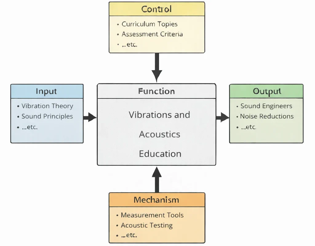
IDEF0 System Functional Decomposition
The IDEF0 framework abstracts vibrations and acoustics education into a structured functional system:
- Inputs (I): Dynamic mechanics principles (harmonic oscillation, Newton's second law, Euler-Lagrange equations) and physical media wave characteristics (elastic modulus E, bulk modulus K, mass density ρ, and acoustic speed c).
- Controls (C): Global accreditation standards (Washington Accord, EUR-ACE, ABET), ISO 10816 machinery vibration evaluation criteria, OSHA occupational noise exposure thresholds, and spectral Nyquist-Shannon sampling limits.
- Mechanisms (M): Triaxial piezoelectric accelerometers, laser Doppler vibrometers (LDV), hemi-anechoic chambers, digital FFT spectral analyzers, modal shakers, and PINN surrogate inference pipelines.
- Outputs (O): Certified structural engineers, calibrated modal parameters, active vibration isolation systems, and optimized acoustic enclosures operating within regulatory sound limits.
Mechanical & Materials Engineering Curriculum Cluster
Select any foundational pillar below to explore related modules across the PREP4UNI.ONLINE Mechanical Engineering series:
Mechanical Engineering
Primary disciplinary framework integrating static equilibrium, dynamic inertial loads, thermal cycles, and machine elements.
Automotive Engineering
Applies quarter-car suspension dynamics, powertrain isolation mounts, and cabin acoustic NVH suppression.
Biomechanical Engineering
Examines high-frequency ultrasound propagation in human tissues and mitigates occupational whole-body vibration.
Control Systems in Mechanical Engineering
Synthesizes active feedback anti-phase noise controllers and electromagnetic actuators to suppress structural resonance.
Fluid Mechanics and Hydraulics
Analyzes flow-induced vortex shedding vibrations, pipe acoustic water-hammer pulses, and aerodynamic turbulence noise.
Manufacturing and Production Engineering
Constructs milling stability lobe diagrams to eliminate regenerative tool chatter and protects foundations from forge shock.
Mechanical Design and CAD
Extracts structural natural frequencies and mode shapes within 3D CAD to isolate assemblies from motor excitation speeds.
Nanotechnology and Advanced Materials
Synthesizes negative-mass acoustic metamaterials and high-loss viscoelastic nanocomposites for sub-wavelength noise blocking.
Robotics and Automation in Mechanical Engineering
Applies zero-vibration input-shaping feedforward filters to eliminate residual arm oscillation during high-speed pick-and-place.
Solid Mechanics: Stress, Strain & Structural Analysis
Converts cyclic dynamic vibration stresses into cumulative fatigue life predictions using S-N curves and Miner's rule.
Thermodynamics and Heat Transfer
Models acoustic pressure wave oscillations driven by combustion heat release (Rayleigh criterion) and thermoacoustic Stirling chillers.
Vibrations and Acoustics
Harmonic oscillator dynamics, modal orthogonality, acoustic wave equations, acoustic impedance, and PINN vibration state identification.
1. Deep Technical Foundations: Structural Dynamics & Oscillatory Systems
1.1 Single Degree of Freedom (SDOF) Formulations
The generalized dynamic equilibrium of a classical viscously damped Single Degree of Freedom (SDOF) mechanical system subjected to an external harmonic excitation force F(t) = F0 cos(ωt) is formulated via d'Alembert's principle:
$$ m \ddot{x}(t) + c \dot{x}(t) + k x(t) = F_0 \cos(\omega t) $$Dividing through by the physical mass m yields the standard normalized canonical differential equation of motion:
$$ \ddot{x}(t) + 2 \zeta \omega_n \dot{x}(t) + \omega_n^2 x(t) = \frac{F_0}{m} \cos(\omega t) $$where the undamped natural frequency ωn and the dimensionless damping ratio ζ are defined by:
$$ \omega_n = \sqrt{\frac{k}{m}}, \qquad \zeta = \frac{c}{c_c} = \frac{c}{2\sqrt{k m}} = \frac{c}{2 m \omega_n} $$For underdamped systems (0 ≤ ζ < 1), the free vibration transient response decays at the damped natural frequency ωd = ωn √(1 − ζ2). The rate of amplitude decay across n successive cycles is measured by the logarithmic decrement δ:
$$ \delta = \frac{1}{n} \ln\left( \frac{x_0}{x_n} \right) = \frac{2 \pi \zeta}{\sqrt{1 - \zeta^2}} $$Under continuous harmonic forcing, the steady-state particular solution exhibits displacement amplitude X and phase lag φ:
$$ X = \frac{F_0 / k}{\sqrt{(1 - r^2)^2 + (2 \zeta r)^2}} = \left(\frac{F_0}{k}\right) M(r, \zeta) $$$$ \phi = \arctan\left( \frac{2 \zeta r}{1 - r^2} \right) $$where r = ω / ωn is the frequency ratio, and M(r, ζ) is the dynamic magnification factor. At resonance (r ≈ 1), the response amplitude is limited entirely by viscous damping: Xres ≈ F0 / (2ζk).
1.2 Multiple Degree of Freedom (MDOF) Systems & Modal Orthogonality
Real engineering structures comprise continuous mass and stiffness distributions discretized into N coordinates. The coupled governing matrix equation of motion is:
$$ \mathbf{M} \ddot{\mathbf{x}}(t) + \mathbf{C} \dot{\mathbf{x}}(t) + \mathbf{K} \mathbf{x}(t) = \mathbf{F}(t) $$where M is the positive-definite symmetric mass matrix, C is the damping matrix, and K is the positive semi-definite stiffness matrix. For undamped free vibration, setting x(t) = Φ ejωt yields the generalized algebraic eigenvalue problem:
$$ \left( \mathbf{K} - \omega_i^2 \mathbf{M} \right) \boldsymbol{\phi}_i = \mathbf{0} $$The roots of the characteristic determinant det(K − ω2M) = 0 define the N natural frequencies ωi, while the non-trivial solutions φi represent the corresponding mode shapes. The eigenvectors satisfy the fundamental modal orthogonality conditions:
$$ \boldsymbol{\phi}_i^T \mathbf{M} \boldsymbol{\phi}_j = 0, \qquad \boldsymbol{\phi}_i^T \mathbf{K} \boldsymbol{\phi}_j = 0 \qquad (\text{for } i \neq j) $$Exploiting modal orthogonality decouples the coupled N-dimensional system into N independent modal coordinates ηi(t) via the modal matrix transformation x(t) = Φ η(t), transforming complex structural dynamics into single-degree-of-freedom solutions.
1.3 Vibration Isolation & Force Transmissibility
When equipment with rotating unbalance generates dynamic force into supporting foundations, resilient isolators (springs and elastomeric pads) attenuate the transmitted force. The force transmissibility Tf (ratio of transmitted force amplitude FT to applied force amplitude F0) is governed by:
$$ T_f = \frac{F_T}{F_0} = \sqrt{\frac{1 + (2 \zeta r)^2}{(1 - r^2)^2 + (2 \zeta r)^2}} $$Effective vibration isolation requires Tf < 1, which occurs strictly when the frequency ratio satisfies:
$$ r = \frac{\omega}{\omega_n} > \sqrt{2} $$For r < √2, adding compliance increases transmitted force above the input force. Crucially, in the isolation zone (r > √2), adding damping ζ actually increases transmissibility at high frequencies while suppressing resonance during startup crossover.
2. Fundamentals of Acoustics: Pressure Waves & Sound Propagation
2.1 The Classical Linear Acoustic Wave Equation
Acoustic disturbances propagate as longitudinal mechanical compressions and rarefactions in elastic fluids. Combining the linearized continuity equation, Euler's momentum equation, and the isentropic equation of state yields the 3D acoustic wave equation for acoustic pressure perturbation p(r, t):
$$ \nabla^2 p - \frac{1}{c^2} \frac{\partial^2 p}{\partial t^2} = 0 $$The thermodynamic speed of sound c in an ideal gas is governed by the Laplace formulation:
$$ c = \sqrt{\frac{\gamma P_0}{\rho_0}} = \sqrt{\gamma R T} $$where γ = cp / cv is the ratio of specific heats, R is the specific gas constant, and T is absolute temperature in kelvins.
2.2 Specific Acoustic Impedance & Boundary Reflection
The characteristic acoustic impedance z0 of a fluid medium defines the ratio of acoustic pressure p to particle velocity u for an undisturbed plane traveling wave:
$$ z_0 = \rho_0 c $$At room temperature (20°C, 1 atm), dry air has z0 ≈ 415 Pa·s/m (Rayls), whereas liquid water has z0 ≈ 1.48 × 10⁶ Rayls. When a plane acoustic wave strikes a planar interface between Medium 1 and Medium 2 at normal incidence, the pressure reflection coefficient Rp and transmission coefficient Tp are:
$$ R_p = \frac{z_2 - z_1}{z_2 + z_1}, \qquad T_p = \frac{2 z_2}{z_2 + z_1} $$When z2 ≫ z1 (e.g., an airborne wave striking a rigid concrete wall), Rp → +1, yielding complete in-phase pressure reflection.
2.3 Logarithmic Sound Pressure & Power Levels
Because the human ear responds logarithmically to acoustic pressure fluctuations spanning six orders of magnitude (20 μPa to 20 Pa), acoustic amplitudes are quantified in decibels (dB):
- Sound Pressure Level (SPL): $$ \text{SPL} = 20 \log_{10}\left( \frac{p_{\text{rms}}}{p_{\text{ref}}} \right) \quad [\text{dB}] $$ where pref = 20 μPa = 2 × 10⁻⁵ Pa is the threshold of human hearing at 1 kHz.
- Sound Power Level (SWL): $$ \text{SWL} = 10 \log_{10}\left( \frac{W}{W_{\text{ref}}} \right) \quad [\text{dB}] $$ where W is acoustic source power in watts and Wref = 10−12 W (1 pW).
2.4 Room Acoustics: Sabine's Reverberation Formulation
In an enclosed room of volume V, acoustic energy undergoes continuous multi-surface reflection until absorbed. The time required for acoustic energy density to decay by 60 dB (reverberation time T60) is formulated via Sabine's classic law:
$$ T_{60} = \frac{0.161 \, V}{A_{\text{total}}} = \frac{0.161 \, V}{\sum_{i} S_i \alpha_i} $$where V is room volume in m3, Si is the surface area of boundary i, and αi is its material-specific sound absorption coefficient (0 ≤ αi ≤ 1).
3. Contemporary Computational Paradigms in Dynamic Systems
High-performance dynamic modeling increasingly leverages neural operator architectures to bypass the meshing bottlenecks and high computational costs of standard Finite Element (FEA) and Boundary Element (BEM) methods.
Physics-Informed Neural Networks (PINNs) for Modal State Estimation
In operating turbine rotors, structural vibration sensors can only be placed on external bearing housings, leaving internal rotor dynamics unmeasured. PINNs embed dynamic equilibrium and wave equations into the network loss function:
$$ \mathcal{L}_{\text{total}}(\theta) = \mathcal{L}_{\text{sensor}}(\theta) + \lambda_{\text{dyn}} \mathcal{L}_{\text{dyn}}(\theta) $$$$ \mathcal{L}_{\text{dyn}}(\theta) = \frac{1}{N_\tau} \sum_{k=1}^{N_\tau} \left\| \mathbf{M} \frac{d^2 \hat{\mathbf{x}}}{dt^2} + \mathbf{C} \frac{d\hat{\mathbf{x}}}{dt} + \mathbf{K} \hat{\mathbf{x}} - \mathbf{F}(t) \right\|^2_{t_k} $$By enforcing Newton's laws across temporal collocation points, the network performs full-field displacement reconstruction and detects unmeasured localized blade cracks without requiring fine temporal meshing.
In vehicle cabin acoustics, Fourier Neural Operators (FNOs) learn mappings directly between 3D acoustic cavity geometry and steady-state pressure field distributions across wide frequency bands, solving Helmholtz radiation equations up to 1,500 times faster than Boundary Element Method (BEM) solvers.
4. Systems Engineering Trade-Off Matrix: Dynamic Attenuation Strategies
Designing dynamic systems requires balancing isolation effectiveness, static deflection limits, operational weight, complexity, and active control stability:
| Control Topology | Primary Advantage | Bottlenecks & Failure Modes | Mitigation Strategy |
|---|---|---|---|
| Passive Elastomeric & Steel Mounts | Zero electrical power input; lowest initial procurement cost; robust structural failsafe capability. | Static sag under heavy loads; material aging/hardening; high transmissibility across resonant crossover. | Dual-rate rubber mounts; mechanical displacement travel stops; environmental ozone-resistant fluoroelastomers. |
| Tuned Mass Dampers (TMDs) | High attenuation of targeted fundamental resonance peaks (up to 80% reduction); passive reliability. | Extremely narrow attenuation bandwidth; de-tuning due to structural modification doubles resonant peaks. | Semi-active variable stiffness TMDs; eddy current damping units; distributed multi-mass damper systems. |
| Active Feedback Vibration Control (AVC) | Adapts dynamically across broadband spectra; attenuates sub-harmonic and non-stationary dynamic forces. | Actuator saturation; high electrical power consumption; closed-loop phase lag causing spillover instability. | H-infinity robust control synthesis; collocated sensor-actuator pairing; hybrid active-passive fail-safe designs. |
| Acoustic Metamaterials & Barriers | Sub-wavelength acoustic blocking; breaks classical mass law for thin structural panels. | Narrow bandgap performance; structural complexity during manufacturing; high acoustic flow-induced shear losses. | Multi-resonant rainbow metamaterial arrays; additive micro-manufacturing; hybrid porous-elastic membranes. |
5. Industrial Systems Case Applications
Aerospace: Rocket Acoustic Launch Loads
At liftoff, rocket engine plumes create violent supersonic turbulence, generating acoustic sound pressure levels exceeding 165 dB within the launch pad flame trench. These acoustic waves reflect upward against the payload fairing, causing intense structural vibration that can damage internal satellites. Launch complexes use high-pressure water deluge suppression systems to inject thousands of gallons of water per minute, converting acoustic pressure energy into water droplet atomization and vaporization.
Automotive: EV Powertrain Tonal Whine
Unlike internal combustion engines with broad masking combustion noise, electric vehicles expose passengers to high-frequency electric motor electromagnetic torque ripple and planetary gearbox tooth mesh whine (1 kHz to 5 kHz). Squeezing gear profiles and micro-geometry topological crowning optimizes contact ratios, while viscoelastic constrained-layer damping (CLD) patches applied to the aluminum motor housing attenuate structural sound radiation.
Precision Manufacturing: Photolithography Isolation
Semiconductor extreme ultraviolet (EUV) lithography scanners pattern silicon wafer features down to sub-3-nanometer tolerances. Ambient seismic ground vibrations, pedestrian footsteps, and HVAC air ducts transmit ground displacements that can ruin exposure alignment. EUV tools sit on active magnetic levitation isolation stages equipped with voice-coil actuators and real-time inertial feedforward sensors, isolating floor disturbances above 0.5 Hz.
6. Interactive Simulation Engine: SDOF Forced Vibration & Resonance
SDOF Forced Vibration & Resonance Simulator
7. Frequently Asked Questions
What is mechanical resonance and why does it cause structural failure?
Why is modal orthogonality essential in structural dynamics?
What governs the boundary between vibration amplification and vibration isolation?
Why do porous materials absorb high-frequency sound while failing at low frequencies?
8. Comprehensive Student Practice Modules
Section 1: Interactive Knowledge Self-Assessment
1. What is the fundamental difference between free and forced vibration?
2. What physical parameters govern the undamped natural frequency of an SDOF system?
3. How does the logarithmic decrement (δ) quantify physical damping?
4. Why is the decibel (dB) scale adopted for sound measurements rather than direct pressure in Pascals?
5. What is the difference between airborne and structure-borne noise propagation?
6. How does a Tuned Mass Damper (TMD) stabilize skyscrapers against wind flutter?
7. What is the physical mechanism behind Active Noise Control (ANC)?
8. How does acoustic impedance mismatch govern sound transmission at an interface?
Section 2: Analytical & Scenario-Based Case Studies
Case 1: Tacoma Narrows Aeroelastic Flutter Catastrophe
Scenario: In 1940, the original Tacoma Narrows suspension bridge suffered catastrophic structural collapse under moderate 68 km/h winds, oscillating in large-amplitude torsional modes.
Engineering Analysis: While historically attributed to simple forced resonance, the collapse was driven by self-excited aeroelastic torsional flutter. Solid plate girders shed alternating Karman vortex sheets that altered dynamic lift and aerodynamic pitching moments. As torsional amplitude grew, aerodynamic forces fed energy into the motion (negative aerodynamic damping), causing structural failure. Modern bridges use aerodynamic open-truss decks to eliminate flow separation and prevent flutter instability.
Case 2: Industrial Centrifugal Compressor Rotating Stall
Scenario: A 5 MW high-pressure natural gas compressor exhibits sharp vibration spikes at 43% of running shaft speed (0.43X RPM) when throttled back during partial capacity operations.
Engineering Analysis: Sub-synchronous vibration at 0.43X indicates rotating aerodynamic stall within the radial diffuser vanes. At low flow, boundary layer separation creates localized stall cells that rotate around the diffuser circumference at roughly half rotor speed, exerting cyclic dynamic pressure pulses on the impeller. Mitigation requires opening anti-surge recycle valves to restore flow margins and redesigning vaneless diffusers to broaden the operational envelope.
Case 3: Semiconductor Cleanroom Fab Micro-Vibration Isolation
Scenario: A transmission electron microscope (TEM) capable of atomic-resolution imaging exhibits horizontal imaging blur whenever vehicular traffic passes on an adjacent roadway 50 meters away.
Engineering Analysis: Soil strata transmit low-frequency Rayleigh surface waves (2 Hz to 10 Hz) into the foundation slab. Passive elastomeric pads amplify these low-frequency displacements because their natural frequency lies near 4 Hz (r ≈ 1). Resolving the blur requires active pneumatic leveling mounts combined with piezoelectric inertial feedforward compensation to isolate vibrations down to 0.5 Hz, satisfying VC-G vibration criteria (< 3 μm/s RMS).
Case 4: Automotive Exhaust Muffler Resonator Tuning
Scenario: A direct-injection turbocharged vehicle produces an objectionable low-frequency interior cabin drone at 120 Hz during highway cruising at 2,400 engine RPM.
Engineering Analysis: For a 4-cylinder engine, the secondary firing order generates acoustic pulsations at f = (RPM / 60) × 2 = (2,400 / 60) × 2 = 80 Hz, while turbocharger blade pass frequencies drive 120 Hz harmonics. Standard reactive mufflers are redesigned to incorporate a side-branch quarter-wave tube or Helmholtz resonator tuned specifically to 120 Hz. At resonance, the side-branch reflects incoming pressure waves with a 180° phase shift, creating zero transmission into the tailpipe.
Case 5: Wind Turbine Drivetrain Planetary Gear Resonance
Scenario: A fleet of 3.5 MW offshore wind turbines experiences premature bearing spalling and gear tooth pitting in the second planetary stage after only 18 months of operation.
Engineering Analysis: Operational modal testing reveals that the gear mesh excitation frequency (fmesh = Nteeth × ωshaft) aligns with the torsional natural mode of the high-speed stage at 428 Hz under high-wind conditions. This continuous resonant torque amplification doubled dynamic tooth contact stresses. The resolution required modifying the planet carrier compliance and adjusting tooth profile crowning to shift the torsional mode away from the operational speed window.
Case 6: Aircraft Auxiliary Power Unit (APU) Acoustic Liner Degradation
Scenario: During ground turnaround operations, passenger cabin ramp noise from an aircraft APU increases by 9 dBA, exceeding airport ground noise regulations.
Engineering Analysis: The APU exhaust duct relies on single-degree-of-freedom (SDOF) acoustic liners composed of perforated composite face sheets backed by a honeycomb core. Inspection reveals that unburnt fuel residue and de-icing fluid mist clogged 35% of the perforation orifices. This reduced the open area ratio (σ), shifting the liner's acoustic impedance away from optimal fluid impedance and drastically reducing sound absorption at target blade-pass frequencies.
Case 7: Subsea Pipeline Vortex-Induced Vibration (VIV) Fatigue
Scenario: A deepwater oil pipeline spanning a seabed canyon exhibits severe cross-flow cyclic displacements, risking fatigue failure at welded joint connections.
Engineering Analysis: Ocean currents moving normal to the pipe generate alternating vortex shedding governed by the Strouhal relationship fs = St · U / D. When shedding frequencies lock onto the pipeline's cross-flow flexural natural frequency, vortex-induced vibration (VIV) triggers sustained limit-cycle oscillations. Installing helical strakes around the outer pipe surface breaks up boundary layer spanwise correlation, suppressing vortex coherence and reducing dynamic lift forces by over 85%.
Section 3: Step-by-Step Quantitative Worked Examples
Worked Problem 1: Free Damped Vibration & Logarithmic Decrement Analysis
A vibrating industrial screening machine is modeled as an SDOF mass-spring-damper system with total mass m = 250 kg and spring stiffness k = 360 kN/m. An initial displacement test is performed. The initial peak displacement is measured at x0 = 15.0 mm. After 5 complete cycles, the peak displacement decays to x5 = 4.2 mm. Determine: (a) the undamped natural frequency ωn, (b) the logarithmic decrement δ, (c) the dimensionless damping ratio ζ, (d) the physical damping coefficient c, and (e) the damped natural frequency fd in Hz.
k = 360,000 N/m, m = 250 kg
ωn = √(k / m) = √(360,000 / 250) = √(1,440) = 37.9473 rad/s
Step 2: Determine logarithmic decrement over 5 cycles:
δ = (1 / n) · ln(x0 / xn) = (1 / 5) · ln(15.0 / 4.2) = 0.20 · ln(3.57143)
ln(3.57143) = 1.27297 ⇒ δ = 0.20 × 1.27297 = 0.25459
Step 3: Calculate the damping ratio ζ:
ζ = δ / √(4π2 + δ2)
4π2 = 4 × (3.14159265)2 = 39.4784
δ2 = (0.25459)2 = 0.06482
ζ = 0.25459 / √(39.4784 + 0.0648) = 0.25459 / √(39.5432) = 0.25459 / 6.28834 = 0.040486 ≈ 0.0405 (4.05%)
Step 4: Compute the critical damping and physical damping coefficient c:
cc = 2 · m · ωn = 2 × 250 × 37.9473 = 18,973.65 N·s/m
c = ζ · cc = 0.040486 × 18,973.65 = 768.17 N·s/m
Step 5: Calculate damped frequency in Hz:
ωd = ωn · √(1 − ζ2) = 37.9473 × √(1 − 0.001639) = 37.9473 × √(0.99836) = 37.9473 × 0.99918 = 37.916 rad/s
fd = ωd / (2π) = 37.916 / 6.283185 = 6.0346 Hz ≈ 6.03 Hz
Worked Problem 2: Rotating Unbalance & Resonant Amplitude Magnification
An electric motor of total mass M = 120 kg is mounted on an elastic foundation with equivalent stiffness k = 1.80 × 10⁶ N/m and damping ratio ζ = 0.08. The internal rotor has mass m0 = 25 kg and an eccentric unbalance center of mass located at radius e = 0.80 mm. The motor runs at an operational speed of N = 1,200 RPM. Evaluate: (a) the undamped natural frequency ωn, (b) the operational driving frequency ω, (c) the dynamic magnification factor M(r, ζ), and (d) the steady-state displacement amplitude X.
ωn = √(k / M) = √(1,800,000 / 120) = √(15,000) = 122.474 rad/s
Step 2: Determine operational excitation frequency and ratio:
ω = 2π · (N / 60) = 2 × 3.14159265 × (1,200 / 60) = 40π = 125.664 rad/s
Frequency ratio: r = ω / ωn = 125.664 / 122.474 = 1.02604
Step 3: Evaluate dynamic magnification for rotating unbalance:
For rotating unbalance, excitation force scales with ω2: F0 = m0 e ω2
F0 = 25 × (0.0008 m) × (125.664)2 = 0.020 × 15,791.4 = 315.83 N
Calculate denominator: D = √[ (1 − r2)2 + (2 ζ r)2 ]
1 − r2 = 1 − (1.02604)2 = 1 − 1.05276 = −0.05276
(1 − r2)2 = (−0.05276)2 = 0.002784
2 ζ r = 2 × 0.08 × 1.02604 = 0.16417
(2 ζ r)2 = (0.16417)2 = 0.026952
D = √(0.002784 + 0.026952) = √(0.029736) = 0.17244
M(r, ζ) = 1 / D = 1 / 0.17244 = 5.799
Step 4: Compute steady-state displacement amplitude X:
Xstatic = F0 / k = 315.83 / 1,800,000 = 1.7546 × 10⁻⁴ m = 0.1755 mm
X = Xstatic · M(r, ζ) = 0.1755 × 5.799 = 1.0175 mm ≈ 1.02 mm
Worked Problem 3: Vibration Isolation Mount Sizing & Force Transmissibility
An industrial air compressor weighing W = 4,905 N (mass m = 500 kg) operates at ω = 180 rad/s (approx. 1,718 RPM). It transmits dynamic harmonic forces into a concrete building floor. Design an elastomeric vibration isolation mounting system with damping ratio ζ = 0.05 such that no more than 10% of the dynamic force is transmitted into the building floor (Transmissibility Tf ≤ 0.10). Determine: (a) the required frequency ratio r, (b) the required mount natural frequency ωn, (c) total required spring stiffness k, and (d) the resulting static deflection δst.
Tf2 = [1 + (2ζr)2] / [ (1 − r2)2 + (2ζr)2 ] ≤ (0.10)2 = 0.010
For light damping (ζ = 0.05) and high isolation (r ≫ √2), the numerator is approximately 1.0, and 1 − r2 ≈ −r2 ⇒ (1 − r2)2 ≈ r4.
Initial estimate: 1 / r2 ≈ 0.10 ⇒ r ≈ √10 ≈ 3.162
Step 2: Solve exact formulation with damping:
At r ≈ 3.35:
Numerator = 1 + (2 × 0.05 × 3.35)2 = 1 + (0.335)2 = 1 + 0.1122 = 1.1122
Denominator = (1 − 3.352)2 + (0.335)2 = (1 − 11.2225)2 + 0.1122 = (−10.2225)2 + 0.1122 = 104.50 + 0.11 = 104.61
Tf2 = 1.1122 / 104.61 = 0.01063 ⇒ Tf = √0.01063 = 0.1031 (10.3%)
Increase slightly to r = 3.42:
Numerator = 1 + (0.342)2 = 1.1170
Denominator = (1 − 11.696)2 + 0.117 = (−10.696)2 + 0.117 = 114.40 + 0.12 = 114.52
Tf = √(1.1170 / 114.52) = √(0.00975) = 0.0987 ≤ 0.10 (9.87% transmitted)
Select target ratio r = 3.42
Step 3: Calculate required natural frequency:
ωn = ω / r = 180 / 3.42 = 52.63 rad/s (8.38 Hz)
Step 4: Compute required total stiffness k:
k = m · ωn2 = 500 × (52.63)2 = 500 × 2,770.08 = 1,385,040 N/m ≈ 1.385 MN/m
(For four corner mounts: keach = 1,385,040 / 4 = 346,260 N/m)
Step 5: Calculate static gravity deflection δst:
δst = (m · g) / k = g / ωn2 = 9.81 / 2,770.08 = 0.003541 m = 3.54 mm
Worked Problem 4: Acoustic Sound Pressure Level (SPL) & Distance Attenuation
An outdoor cooling tower fan acts as an omnidirectional point acoustic source on a flat concrete foundation slab (hemispherical radiation, directivity factor Q = 2). The sound pressure level measured at a distance r1 = 5.0 m is SPL1 = 88.0 dB (ref: 20 μPa). Assuming standard atmospheric air (ρ0 = 1.20 kg/m3, c = 343 m/s) and neglecting air absorption: (a) calculate the acoustic root-mean-square pressure prms,1 at 5 m, (b) determine the total sound power W radiated in Watts and its Sound Power Level (SWL), and (c) calculate the SPL at the property boundary line r2 = 40.0 m.
SPL1 = 20 log10(prms,1 / pref) = 88.0 dB
log10(prms,1 / pref) = 88.0 / 20 = 4.40
prms,1 / pref = 104.40 = 25,118.86
prms,1 = 25,118.86 × (20 × 10−6 Pa) = 0.50238 Pa ≈ 0.502 Pa
Step 2: Determine sound intensity and total radiated acoustic power:
Characteristic impedance: z0 = ρ0 c = 1.20 × 343 = 411.6 Pa·s/m
Acoustic intensity: I1 = prms,12 / z0 = (0.50238)2 / 411.6 = 0.25238 / 411.6 = 6.1317 × 10⁻⁴ W/m2
For hemispherical radiation, area: A1 = 2π r12 = 2 × 3.14159265 × (5.0)2 = 50π = 157.08 m2
Radiated Sound Power: W = I1 · A1 = (6.1317 × 10−4) × 157.08 = 0.09632 W (96.32 mW)
SWL = 10 log10(W / 10−12 W) = 10 log10(9.632 × 10¹⁰) = 10 × 10.9837 = 109.84 dB
Step 3: Calculate SPL at r2 = 40.0 m via inverse square law:
For hemispherical geometric spreading: SPL2 = SPL1 − 20 log10(r2 / r1)
r2 / r1 = 40.0 / 5.0 = 8.0
20 log10(8.0) = 20 × 0.90309 = 18.06 dB
SPL2 = 88.0 − 18.06 = 69.94 dB ≈ 69.9 dB
Worked Problem 5: Room Reverberation Time & Acoustic Absorption Sizing
A university engineering auditorium has dimensions length L = 20.0 m, width W = 15.0 m, and height H = 6.0 m. The untreated enclosure consists of: hard plaster walls (Swalls = 420 m2, α1 = 0.04), concrete floor (Sfloor = 300 m2, α2 = 0.02), and gypsum board ceiling (Sceil = 300 m2, α3 = 0.05) evaluated at 1 kHz. Calculate: (a) the untreated reverberation time T60, (b) the target reverberation time for speech intelligibility (target ≈ 0.75 s), and (c) the area of acoustic wall panels (αpanel = 0.85) required to replace the plaster to achieve the target.
V = 20.0 × 15.0 × 6.0 = 1,800 m3
Plaster absorption: A1 = 420 × 0.04 = 16.8 m2 Sabins
Floor absorption: A2 = 300 × 0.02 = 6.0 m2 Sabins
Ceiling absorption: A3 = 300 × 0.05 = 15.0 m2 Sabins
Total initial absorption: Ainitial = 16.8 + 6.0 + 15.0 = 37.8 m2 Sabins
Step 2: Compute untreated reverberation time via Sabine's equation:
T60,initial = (0.161 · V) / Ainitial = (0.161 × 1,800) / 37.8 = 289.8 / 37.8 = 7.667 seconds
Step 3: Calculate required total absorption for target T60 = 0.75 s:
Atarget = (0.161 · V) / T60,target = 289.8 / 0.75 = 386.4 m2 Sabins
Required net absorption increase: ΔA = 386.4 − 37.8 = 348.6 m2 Sabins
Step 4: Determine required acoustic panel surface area Spanel:
Replacing plaster (α1 = 0.04) with acoustic panels (αpanel = 0.85) yields a net gain per unit area:
Δα = αpanel − α1 = 0.85 − 0.04 = 0.81 Sabins/m2
Spanel = ΔA / Δα = 348.6 / 0.81 = 430.37 m2
Because total wall area is 420 m2, wall coverage alone is insufficient (430.4 > 420).
Adjust treatment: Cover 250 m2 of walls and 183 m2 of ceiling with panels (αceil,gain = 0.85 − 0.05 = 0.80):
Wall gain: 250 × 0.81 = 202.5 Sabins
Ceiling gain: 183 × 0.80 = 146.4 Sabins
Total gain = 202.5 + 146.4 = 348.9 Sabins ⇒ Achieved T60 = 289.8 / (37.8 + 348.9) = 289.8 / 386.7 = 0.749 s
Worked Problem 6: Helmholtz Resonator Acoustic Intake Tuning
An internal combustion engine air intake manifold produces an aggressive acoustic standing wave at fres = 140 Hz. A side-branch Helmholtz resonator is designed to cancel this frequency. The resonator neck has an inner diameter dneck = 40 mm (radius r = 0.02 m) and physical length Lneck = 65 mm. Taking the speed of sound in air as c = 343 m/s: (a) calculate the effective acoustic neck length Leff including end corrections, and (b) determine the required resonator acoustic cavity volume V in liters.
S = π r2 = 3.14159265 × (0.020)2 = 3.14159 × 0.0004 = 1.25664 × 10⁻³ m2
Step 2: Calculate effective neck length with flanged/unflanged end corrections:
Inner end opening into cavity: ΔLin ≈ 0.85 r
Outer end opening flush into duct: ΔLout ≈ 0.85 r
Total end correction: ΔL = 1.70 r = 1.70 × 0.020 = 0.034 m (34.0 mm)
Leff = Lneck + ΔL = 0.065 + 0.034 = 0.099 m (99.0 mm)
Step 3: Formulate Helmholtz resonance relationship:
fres = (c / 2π) · √[ S / (V · Leff) ]
Square both sides:
fres2 = [c2 / (4π2)] · [ S / (V · Leff) ]
Rearrange to solve for cavity volume V:
V = [ c2 · S ] / [ 4π2 · fres2 · Leff ]
Step 4: Calculate numerical volume V:
c2 = (343)2 = 117,649 m2/s2
Numerator = 117,649 × (1.25664 × 10−3) = 147.843 m5/s2
4π2 = 39.4784
fres2 = (140)2 = 19,600 s−2
Denominator = 39.4784 × 19,600 × 0.099 = 773,776.6 × 0.099 = 76,603.88 m·s−2
V = 147.843 / 76,603.88 = 1.9300 × 10⁻³ m3
Convert to liters (1 m3 = 1,000 L):
V = 1.9300 × 10−3 × 1,000 = 1.930 Liters