Robotics and Automation in Mechanical Engineering Explained: Robots, Control Systems, Industrial Automation

Target Level: Undergraduate Engineering / Adv STEM

Estimated Study Time: 75–85 Minutes

Curricular Framework: Washington Accord / EUR-ACE

Principal Editor: Dr. Jacob Gan, PhD (Mich)

Robotics and automation in mechanical engineering is the science of embodying computational intelligence into multi-body physical systems. It unifies forward and inverse kinematics, non-linear multi-body dynamics, gear transmission inertia matching, structural compliance, and sensor-actuator feedback control to execute precise, high-speed, and safe mechanical work.

Executive Curricular Takeaways:

Kinematics & Geometric Mapping: Formulate coordinate frame transformations using Denavit-Hartenberg (D-H) 4×4 homogeneous matrices, analytical inverse kinematics, and workspace reach envelopes.
Differential Motion & Statics: Derive the geometric Jacobian matrix, resolve joint velocities to Cartesian task rates, map wrench forces via virtual work, and identify boundary and interior singularities.
Dynamic Equations of Motion: Formulate multi-link dynamics via the Lagrange-Euler energy method, evaluate mass-inertia matrices, centrifugal and Coriolis torque vectors, and calculate optimal actuator gear ratio matching.

IDEF0 diagram of Robotics and Automation in Mechanical Engineering Education showing robot kinematics and control theory as inputs, shaped by curriculum topics and assessment criteria, enabled by robotic platforms and programming tools, producing skilled graduates and automated solutions.

Figure 1.0: IDEF0 Functional Architecture of Robotics & Automation Education (PREP4UNI.ONLINE Curricular Blueprint).

IDEF0 (Input-Control-Output-Mechanism) Systems Decomposition:

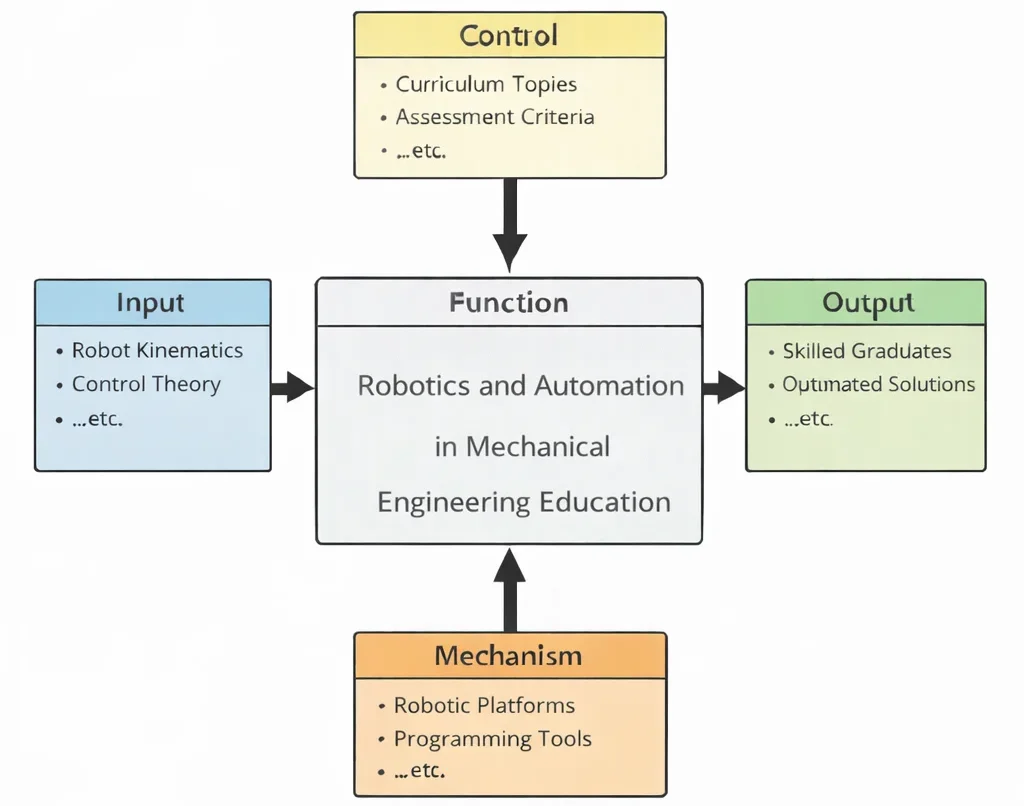
Inputs (Left): Multi-link kinematic topologies, target tool-center-point (TCP) trajectories, payload mass envelopes, sensor telemetry, and dynamic environmental disturbance profiles.
Controls (Top): Washington Accord/EUR-ACE quality criteria, ISO 10218-1/2 industrial robot safety mandates, ISO/TS 15066 collaborative robot thresholds, and cycle time limits.
Mechanisms (Bottom): 6-axis articulated arms, harmonic drive gearboxes, absolute optical encoders, 6-axis wrist force-torque transducers, ROS2/MoveIt motion planners, and real-time EtherCAT fieldbuses.
Outputs (Right): Certified collision-safe manipulator cells, optimized singularity-free toolpaths, validated dynamic load profiles, and industry-ready automation engineers.

Mechanical & Robotics Engineering Curriculum Cluster

Select any foundational pillar below to explore related modules across the PREP4UNI.ONLINE Mechanical Engineering series:

Core Disciplines

Mechanical Engineering

Provides kinematic synthesis, static force balances, actuator thermal ratings, and dynamic stability for automated systems.

Self-Driving AGVs

Automotive Engineering

Deploys SLAM trajectory planning on autonomous industrial mobile carts and integrates drive-by-wire electric steering.

Surgical Robotics

Biomechanical Engineering

Translates human hand tremor cancellation algorithms to laparoscopic surgical telemanipulators and powered gait orthotics.

Servomotor Algorithms

Control Systems in Mechanical Engineering

Executes digital computed-torque control, Kalman state estimation, and dynamic impedance feedback for robotic touch.

Heavy Hydraulics

Fluid Mechanics and Hydraulics

Drives high-torque hydraulic actuators on heavy construction manipulators and operates pneumatic vacuum suction cups.

Factory Automation

Manufacturing and Production Engineering

Orchestrates robotic CNC tendering, synchronized multi-arm automotive spot welding lines, and automated packaging cells.

Arm Assembly CAD

Mechanical Design and CAD

Designs 6-DOF hollow arm castings to house internal wiring, gearboxes, and custom payload end-effector mounts.

Tactile Nanotech

Nanotechnology and Advanced Materials

Equips grippers with piezoresistive graphene pressure sensors and integrates shape memory alloy micro-actuators.

Current Topic

Robotics and Automation in Mechanical Engineering

Forward and inverse kinematics, Denavit-Hartenberg frames, path trajectory planning, dynamic torques, and automation.

Cantilever Bending

Solid Mechanics: Stress, Strain & Structural Analysis

Calculates link deflection and torsional shaft windup during emergency high-inertia stops to maintain tool positional repeatability.

Joint Heat Rejection

Thermodynamics and Heat Transfer

Dissipates continuous copper coil Joule heating in compact robot joints to prevent thermal demagnetization and stall.

Residual Settling

Vibrations and Acoustics

Applies input shaping and notch filtering to eliminate end-effector residual oscillations during high-speed pick maneuvers.

Robotics and Automation in Mechanical Engineering futuristic laboratory showing multi-axis articulated robots, autonomous drones, and digital inspection interfaces.

Figure 2.0: Cyber-physical automation studio: high-speed multi-axis kinematic manipulation, real-time dynamic tracking, and collaborative human-robot work cells.

Deep Technical Foundations: Analytical Kinematics & Multi-Body Manipulator Dynamics

Robotic manipulation bridges spatial geometry with dynamic balance. Achieving millimeter-level tracking accuracy under rapid acceleration requires modeling kinematic frame chains, resolving Jacobian singularities, and formulating multi-link equations of motion.

1. Forward Kinematics: The Denavit-Hartenberg (D-H) Formulation

Spatial relationships between adjacent coordinate frames (from link i−1 to link i) are established by four standard D-H parameters: link length a_i−1, link twist α_i−1, link offset d_i, and joint angle θ_i. The resulting homogeneous transformation matrix ⁱ⁻¹T_i is expressed as:

$${}^{i-1}\mathbf{T}_i = \begin{bmatrix} \cos\theta_i & -\sin\theta_i\cos\alpha_{i-1} & \sin\theta_i\sin\alpha_{i-1} & a_{i-1}\cos\theta_i \\ \sin\theta_i & \cos\theta_i\cos\alpha_{i-1} & -\cos\theta_i\sin\alpha_{i-1} & a_{i-1}\sin\theta_i \\ 0 & \sin\alpha_{i-1} & \cos\alpha_{i-1} & d_i \\ 0 & 0 & 0 & 1 \end{bmatrix}$$

Compounding individual link transformations from base frame (0) to end-effector tool-center-point (n) establishes the total forward kinematic map:

$${}^0\mathbf{T}_n = {}^0\mathbf{T}_1 \cdot {}^1\mathbf{T}_2 \cdot {}^2\mathbf{T}_3 \dots {}^{n-1}\mathbf{T}_n = \begin{bmatrix} \mathbf{R}_{3\times 3} & \mathbf{P}_{3\times 1} \\ \mathbf{0}_{1\times 3} & 1 \end{bmatrix}$$

2. Differential Kinematics, Jacobian Matrix & Singularity Analysis

The geometric Jacobian matrix J(q) maps joint velocity vectors q̇ to Cartesian end-effector linear velocity v and angular velocity ω:

$$\mathbf{\dot{x}} = \begin{bmatrix} \mathbf{v} \\ \boldsymbol{\omega} \end{bmatrix} = \mathbf{J}(\mathbf{q}) \mathbf{\dot{q}} = \begin{bmatrix} \mathbf{J}_v(\mathbf{q}) \\ \mathbf{J}_\omega(\mathbf{q}) \end{bmatrix} \mathbf{\dot{q}}$$

By the principle of virtual work, the transpose of the Jacobian matrix maps external Cartesian contact wrenches (forces and moments) F_ext to required joint holding torques τ:

$$\boldsymbol{\tau} = \mathbf{J}^T(\mathbf{q}) \mathbf{F}_{\text{ext}}$$

Kinematic singularities occur when the Jacobian matrix loses rank (det(J) = 0 for square Jacobians). At singular configurations, the manipulator loses one or more degrees of freedom, and inverse kinematic velocity solutions command infinite joint rates (Δq̇ → ∞).

3. Multi-Body Manipulator Dynamics: The Lagrange-Euler Formulation

The closed-form equations of motion for an n-link articulated manipulator operating under gravitational and inertial forces are derived via the Lagrangian L = K − P:

$$\mathbf{M}(\mathbf{q})\mathbf{\ddot{q}} + \mathbf{C}(\mathbf{q},\mathbf{\dot{q}})\mathbf{\dot{q}} + \mathbf{G}(\mathbf{q}) = \boldsymbol{\tau}$$

where M(q) is the symmetric, positive-definite n×n mass-inertia matrix, C(q, q̇)q̇ is the n×1 vector of centrifugal and Coriolis torques, G(q) is the n×1 gravitational torque vector, and τ is the n×1 vector of generalized joint actuator torques.

Contemporary Computational Paradigms in Robotics & Automation

Modern industrial robotics has moved from rigid, pre-taught position playback to dynamic perception, physics-based simulation, and cloud-coordinated execution:

Physics-Informed Neural Networks for Dynamic Compensation

PINNs combine multi-body rigid dynamics with real-time drive current telemetry to estimate complex joint friction (Stribeck curve, viscous damping, and cable hysteresis). Feedforward neural networks cancel non-linear friction disturbances in real time, improving trajectory tracking precision by over 80%.

Model Predictive Trajectory Planning (NMPC)

Non-linear Model Predictive Control solves real-time Quadratic Programming (QP) optimization problems over a moving time horizon. NMPC plans time-optimal, collision-free Cartesian trajectories while strictly enforcing joint torque limits, motor voltage boundaries, and ISO 15066 collaborative speed thresholds.

Digital Twins & Hardware-in-the-Loop Simulation

Virtual commissioning environments (NVIDIA Isaac Sim, Gazebo) connect industrial PLCs and robot controllers over deterministic fieldbuses (EtherCAT, PROFINET). Complete factory assembly cells are tested, collision-checked, and cycle-time optimized in software before physical hardware installation.

Systems Engineering Trade-off Matrix

Designing robotic manipulation cells requires balancing structural rigidity, payload capacity, trajectory velocity, and collision safety:

Robotic Architecture / Design Choice	Primary Engineering Advantage	Bottlenecks & Failure Modes	Mitigation & Control Strategy
High Gear Ratio Reduction (N > 100:1)	Amplifies joint motor torque; matches high-inertia mechanical links; enables compact electric motor packaging.	Reflects high mechanical friction and torsional compliance; magnifies gear backlash; introduces flex-spline hysteresis in harmonic drives.	Implement dual-encoder feedback (measuring motor shaft and joint output directly); utilize zero-backlash cycloidal speed reducers.
Direct-Drive Arm Architecture (N = 1:1)	Eliminates mechanical gear backlash and transmission friction; provides high dynamic bandwidth and backdrivability.	Requires large, heavy high-torque torque motors; low mechanical advantage causes high motor current draw and thermal heat dissipation.	Deploy water-cooled frameless torque motors; optimize link structural mass using topological carbon fiber composite casting.
Collaborative Robot (Cobot) Compliance	Enables safe fenceless human-robot collaboration; compliant joint torque sensors detect unintended collisions instantly.	Restricted payload capacity (< 15 kg); low maximum Cartesian speed (≤ 250 mm/s per ISO 10218) limits high-volume throughput.	Implement multi-zone safety LiDAR scanners: run at high speed when humans are absent, transitioning dynamically to safe mode upon approach.
Parallel Delta Robot Topology	Stationary base-mounted actuators reduce moving mass to near zero; delivers extreme accelerations (> 15g) in pick-and-place.	Severely restricted, shallow cylindrical workspace envelope; complex multi-loop inverse kinematics with numerous singular zones.	Deploy analytical algebraic singularity mapping; constrain pick-and-place motions strictly within central dextrous workspace boundaries.

Cross-Sector Industrial Case Studies

Automotive BiW Resistance Spot Welding

Automotive Body-in-White (BiW) lines utilize heavy articulated 6-axis robots carrying 150-kg servo-electric weld guns. Trajectory controllers run model-based vibration suppression filters, enabling 2000 spot welds per vehicle with positioning repeatability within ±0.05 mm.

Semiconductor Wafer Vacuum Handlers

SCARA-type atmospheric and high-vacuum robotic transfer arms transport 300-mm silicon wafers between photolithography vacuum chambers. Direct-drive magnetically levitated joints eliminate lubricants, preventing particulate contamination in ISO Class 1 cleanrooms.

Aerospace Robotic Drilling & Fastening

Drilling fastener holes in titanium-composite aircraft fuselages requires 3 kN of normal clamping force. Robotic end-effectors incorporate pressure-foot load cells and secondary laser vision trackers, compensating for structural arm deflection in real time to maintain hole perpendicularity within 0.5 degrees.

Warehouse Autonomous Mobile Robots (AMRs)

Logistics fulfillment centers deploy fleets of differential-drive AMRs. Sensor-fusion algorithms combine 2D LiDAR simultaneous localization and mapping (SLAM) with wheel odometry and 3D depth cameras, moving 1.5-ton pallet racks along dynamic obstacle-free paths.

Interactive Simulation: 2-DOF Robotic Arm Kinematics & Reach Engine

Evaluate real-time forward kinematics, coordinate transformations, and reach boundaries for a two-link planar robotic manipulator using our verified zero-crash canvas architecture.

Interactive 2-DOF Robotic Arm Kinematics Simulator

STATUS: ACTIVE SOLVER

Simulates planar forward kinematics for a two-link articulated arm (L₁ = 1.2 m, L₂ = 0.8 m). Adjust joint rotation angles to observe spatial end-effector coordinate positioning and workspace boundary reach.

Joint 1 Angle (θ₁): 45°

Joint 2 Angle (θ₂): 30°

End-Effector X

1.06 m

End-Effector Y

1.62 m

Scalar Reach (R)

1.93 m

Max Reach Limit

2.00 m

Manipulator Link 1 & Link 2 Maximum Workspace Reach Boundary (2.0 m) Tool Center Point (TCP)

Frequently Asked Questions: Industrial Robotics & Autonomous Systems

1. How do forward kinematics and inverse kinematics differ in complexity?

Forward kinematics is a deterministic, closed-form algebraic mapping that calculates the Cartesian position and orientation of the end-effector given known joint angles ([x, y, z, α, β, γ]^T = f(q)); it always yields a single unique geometric solution. Inverse kinematics determines the required joint angles to achieve a desired Cartesian tool pose (q = f⁻¹(x)). It involves non-linear trigonometric equations that often produce multiple mathematical solutions (e.g., elbow-up vs. elbow-down configurations) or no solution if the target lies outside the reachable workspace envelope.

2. What is a robot kinematic singularity, and how do controllers avoid it?

A kinematic singularity occurs when the manipulator's joint axes line up such that the geometric Jacobian matrix loses full rank (det(J) = 0). In this configuration, the robot loses the ability to move in one or more Cartesian directions, and commanding velocity in that direction requires infinite joint speeds (q̇ = J⁻¹ẋ → ∞). Controllers avoid singularities using Damped Least-Squares (Levenberg-Marquardt) algorithms, which trade small Cartesian tracking offsets to maintain bounded joint velocities.

3. Why is inertia matching critical in selecting robot actuator gear ratios?

In a geared joint drive, the load inertia reflected back to the motor shaft scales inversely with the square of the gear reduction ratio (J_refl = J_L / N²). Total equivalent inertia is J_eq = J_m + J_L / N². Setting the gear ratio to the optimal inertia-matched condition N_opt = √(J_L / J_m) maximizes angular acceleration for a given motor torque capacity, maximizing pick-and-place dynamic responsiveness.

4. What safety standards govern collaborative human-robot interaction (Cobots)?

Industrial cobots are certified under ISO 10218-1/2 and ISO/TS 15066 safety directives. These standards establish four collaborative operational modes: Safety-Rated Monitored Stop, Hand Guiding, Speed and Separation Monitoring (using safety laser area scanners), and Power and Force Limiting (PFL). Under PFL mode, embedded joint torque sensors restrict transient collision force and dynamic impact energy below biomechanical pain-onset thresholds across 29 specific human body zones.

5. How does the Jacobian transpose relate joint torques to end-effector contact forces?

Applying the principle of virtual work, the virtual work done in joint space (δW = τ^T δq) must balance the virtual work done in Cartesian task space (δW = F_ext^T δx). Because differential motion satisfies δx = J δq, substituting yields: $$\boldsymbol{\tau}^T \delta\mathbf{q} = \mathbf{F}_{\text{ext}}^T \mathbf{J}\delta\mathbf{q} \quad \Rightarrow \quad \boldsymbol{\tau} = \mathbf{J}^T(\mathbf{q}) \mathbf{F}_{\text{ext}}$$ This formulation enables impedance control and force-guiding without requiring individual joint torque transducers at every axis.

6. What causes gear backlash in articulated robot joints, and how is it mitigated?

Backlash is the clearance play between mating gear teeth required to prevent binding and accommodate lubrication. In serial manipulators with long link extensions, a small angular backlash at Joint 1 is multiplied by link length, resulting in millimeter-level positioning jitter at the tool. It is eliminated by using zero-backlash strain-wave Harmonic Drives, preloaded cycloidal speed reducers, or dual-pinion electronically preloaded drive systems.

7. What is the fundamental difference between SCARA and Delta robot architectures?

A SCARA (Selective Compliance Articulated Robot Arm) is a 4-DOF serial mechanism that is rigid in the vertical Z-axis but compliant in the horizontal X-Y plane, suited for vertical PCB insertion. A Delta robot is a parallel mechanism featuring three closed kinematic loops driving a shared end-effector plate from heavy stationary base-mounted motors, enabling ultra-fast pick-and-place accelerations (> 15g).

8. How do industrial robots communicate over real-time deterministic fieldbuses?

Modern robot automation cells use real-time Industrial Ethernet protocols (such as EtherCAT, PROFINET IRT, and Ethernet/IP). These protocols bypass standard non-deterministic TCP/IP stack overhead, utilizing dedicated hardware framing to synchronize multi-axis servo drives, machine vision systems, and safety interlocks with cycle jitter under 1 microsecond.

Student Practice & Accreditation Assessment Modules

Section 1: Interactive Knowledge Self-Assessment

Q1: Formulate how cumulative positioning errors propagate along open serial kinematic chains.

In serial manipulators, each link frame is positioned relative to the preceding joint frame. Angular machining tolerances, bearing clearances, and gear backlash at Joint 1 deflect the entire downstream arm. The Cartesian displacement error at the tool center point scales linearly with distance: $$\Delta X_{\text{TCP}} \approx \sum_{i=1}^n \left( \Delta\theta_i \times \mathbf{r}_{i,\text{TCP}} + \Delta\mathbf{d}_i \right)$$ Consequently, serial robots require high joint manufacturing precision to prevent compounded tip error.

Q2: Differentiate between repeatability and absolute accuracy in industrial manipulators.

Repeatability: The ability of a manipulator to return to the exact same taught coordinate position under repeated cycles (typically ±0.02 mm in modern industrial arms).
Absolute Accuracy: The ability of a robot to move to a mathematically programmed Cartesian coordinate without prior physical teaching (often ±0.5 to 2.0 mm due to link compliance, thermal expansion, and kinematic parameter manufacturing variances).

Q3: Why do industrial robots experience wrist singularities, and how are they identified?

In standard 6-axis articulated robots with spherical wrists (Axes 4, 5, 6 intersecting at a single point), a wrist singularity occurs whenever Axis 4 and Axis 6 become collinear (Joint Angle θ₅ = 0°). In this alignment, the wrist loses one rotational degree of freedom; commanding an orientation rate about the orthogonal axis requires infinite, opposing angular velocities on Joint 4 and Joint 6.

Q4: How does dynamic operational space impedance control differ from pure position control?

Pure position control enforces a pre-computed geometric trajectory regardless of contact forces, which can damage workpieces or trip motor overcurrent alarms during mechanical assembly. Impedance control programs the robot to act as a virtual mass-spring-damper system: $$\mathbf{M}_d (\mathbf{\ddot{x}} - \mathbf{\ddot{x}}_d) + \mathbf{D}_d (\mathbf{\dot{x}} - \mathbf{\dot{x}}_d) + \mathbf{K}_d (\mathbf{x} - \mathbf{x}_d) = \mathbf{F}_{\text{contact}}$$ allowing the manipulator to yield smoothly in response to external contact forces.

Q5: Why is input shaping vibration control applied to flexible robotic manipulators?

Long, lightweight robotic arms possess low structural natural frequencies that oscillate when subjected to rapid step accelerations. Input shaping convolves the input command trajectory with a sequence of discrete impulses tuned to the structural resonance period. The second impulse generates a vibration wave exactly 180 degrees out of phase with the first impulse, canceling residual oscillations upon move completion.

Q6: What causes centrifugal and Coriolis torque coupling in multi-axis robotic arms?

In multi-body rotating systems, the velocity of an outer link depends on the angular velocity of preceding inner links. In the Lagrange-Euler formulation, the Coriolis and centrifugal matrix terms: $$C_{ij}(\mathbf{q}, \mathbf{\dot{q}}) = \sum_{k=1}^n \frac{1}{2} \left( \frac{\partial M_{ij}}{\partial q_k} + \frac{\partial M_{ik}}{\partial q_j} - \frac{\partial M_{jk}}{\partial q_i} \right) \dot{q}_k$$ arise from dynamic cross-coupling. Moving Joint 1 while Joint 2 is rotating induces Coriolis cross-torques that must be balanced by joint motor drivers.

Q7: Differentiate between LiDAR-based SLAM and visual SLAM for Autonomous Mobile Robots (AMRs).

LiDAR SLAM uses time-of-flight laser scans to build 2D/3D geometric point clouds, operating independently of ambient lighting conditions and providing high measurement range accuracy. Visual SLAM uses stereo or RGB-D cameras to track optical feature keypoints across consecutive video frames, offering rich texture and semantic object identification at lower hardware cost, but remaining sensitive to shadows, glare, and featureless surfaces.

Q8: Formulate why joint torque sensors enable fenceless collaborative operation.

Standard motor current sensing measures combined gear friction, inertia, and payload forces, making it difficult to isolate small external human contact forces. Strain-gauge joint torque sensors mounted directly on the output side of joint reducers measure external contact torques directly: $$\boldsymbol{\tau}_{\text{contact}} = \boldsymbol{\tau}_{\text{measured}} - \boldsymbol{\tau}_{\text{model}}(\mathbf{q}, \mathbf{\dot{q}}, \mathbf{\ddot{q}})$$ enabling collision detection within 5 milliseconds to safely stop the robot.

Section 2: Analytical & Scenario-Based Case Studies

Case Study 2.1: Wrist Singularity Lockup and Trajectory Deviation in Automotive Sealing AUTOMOTIVE AUTOMATION

Scenario: A 6-axis articulated robot applying adhesive sealant along a car windshield frame produced uneven, discontinuous sealant beads and tripped axis overspeed alarms at the upper corner radius.

Engineering Evaluation:
1. Kinematic Alignment: Trajectory planning commanded the tool to maintain a constant normal angle while traversing across the roofline. At the upper corner, Joint 5 passed through zero degrees (θ₅ = 0°), aligning Joint 4 and Joint 6 axes.
2. Singularity Dynamics: The inverse Jacobian determinant dropped to zero: $$\det(\mathbf{J}) \approx 0$$ The controller commanded Joint 4 to reverse at 350 deg/s to satisfy orientation constraints, exceeding motor torque limits. The robot dropped out of coordinated path tracking, causing adhesive bead pooling and surface defects.
Corrective Engineering Action: Reposition the robot mounting pedestal 150 mm lower relative to the car body, tilting the tool mounting bracket by 15 degrees. This introduces an angular bias that ensures Joint 5 maintains θ₅ ≥ 12° throughout the sealing path, bypassing the singular zone.

Case Study 2.2: Harmonic Drive Tooth Spalling from Rapid Emergency Stops in Palletizing Cells DRIVE MECHANICS

Scenario: A heavy box-palletizing robot carrying a 50-kg payload suffered mechanical drive failure on Joint 2 after 9 months. Teardown revealed stripped teeth on the internal flexspline ring of its 160:1 harmonic speed reducer.

Engineering Evaluation:
1. Inertial Braking Loads: The safety light curtain was tripped repeatedly by forklift operators entering loading zones, initiating hard Category 0 emergency stops (instantaneous mechanical brake engagement).
2. Dynamic Torque Amplification: Decelerating a fully extended 50-kg payload from 2.0 m/s in 0.08 seconds generated dynamic stopping torques: $$\tau_{\text{dyn}} = J_{\text{total}} \cdot \alpha_{\text{stop}} \approx 1450 \text{ N}\cdot\text{m}$$ exceeding the 850 N·m repeated peak torque rating of the harmonic reducer, causing fatigue tooth shear.
Corrective Engineering Action: Reprogram emergency circuits to execute Category 1 controlled stops: joint servo drives apply maximum regenerative electrical braking torque for 0.25 seconds before engaging mechanical friction brakes. Upgrade Joint 2 to a high-capacity cycloidal drive capable of withstanding 500% shock overloads.

Case Study 2.3: Thermal Kinematic Drift in High-Precision Silicon Wafer Cleanroom Transfer SEMICONDUCTOR ROBOTICS

Scenario: A cleanroom vacuum transfer robot handling 300-mm silicon wafers began dropping wafers at Process Chamber 3 after 6 hours of continuous wafer processing.

Engineering Evaluation:
1. Thermal Conduction: Radiant heat from the 450°C chemical vapor deposition furnace warmed the robot's aluminum end-effector and forearm links to 62°C (ΔT = +40°C).
2. Kinematic Extension: Thermal expansion (α_Al = 23 × 10⁻⁶ /°C) of the 600-mm forearm link caused linear expansion: $$\Delta L = L_0 \cdot \alpha \cdot \Delta T = 0.600 \cdot (23 \times 10^{-6}) \cdot (40) \approx 0.552 \text{ mm}$$ Because vacuum end-effector positioning tolerances were ±0.15 mm, the 0.55-mm thermal drift caused mechanical interference with chamber cassette guide pins.
Corrective Engineering Action: Re-fabricate the end-effector arm from carbon-fiber-reinforced cyanate ester composite with near-zero thermal expansion (α < 0.5 × 10⁻⁶ /°C). Install thermal isolator ceramic spacers at the wrist flange to block heat conduction into the link structure.

Case Study 2.4: Mechanical Chatter and Surface Rippling in High-Feed Robotic Machining ROBOTIC MACHINING

Scenario: A 6-axis articulated robot outfitted with a high-speed milling spindle produced severe chatter marks (Ra > 12 μm) while trimming edge contours on aluminum aerospace wing skins.

Engineering Evaluation:
1. Low Structural Stiffness: Serial robotic arms possess Cartesian structural stiffness of approximately 1.0–2.5 N/μm, compared to > 50 N/μm for dedicated CNC gantry machine tools.
2. Process Dynamics: The 4-flute end mill rotating at 12,000 RPM generated an 800-Hz cutting force excitation that matched the second flexural torsional resonance mode of Robot Axis 3, driving the tool into regenerative chatter.
Corrective Engineering Action: Deploy an external optical tracking system (laser tracker reading reflective retroreflectors on the spindle head) that executes secondary high-bandwidth position feedback, bypassing joint compliance. Reprogram the toolpath to utilize climb milling at spindle speeds tuned via stability lobe diagrams to avoid structural resonance.

Case Study 2.5: Uncontrolled Slip and Breakage in High-Speed Pneumatic Robotic Grippers END-EFFECTOR DESIGN

Scenario: An automated packaging line delta robot operating at 120 picks per minute dropped glass beverage bottles during high-acceleration transfer maneuvers (> 8g).

Engineering Evaluation:
1. Inertial Force Balance: During rapid direction reversal, the inertial stripping force acting on the 0.5-kg bottle reached: $$F_{\text{inertia}} = m \cdot a = 0.5 \text{ kg} \cdot (8 \cdot 9.81 \text{ m/s}^2) \approx 39.24 \text{ N}$$ 2. Friction Limits: The pneumatic gripper applied 120 N of clamping force through smooth aluminum jaws. With friction coefficient μ = 0.25, total frictional holding force was F_fric = 2 · μ · F_clamp = 2(0.25)(120) = 60 N. When bottles had surface condensation, friction dropped to μ = 0.12 (F_fric = 28.8 N < F_inertia), causing slip.
Corrective Engineering Action: Replace flat aluminum fingers with form-fitting urethane-molded jaws matching bottle neck geometry. The mechanical interlock supports inertial loads through direct bearing reaction rather than surface friction alone.

Case Study 2.6: Fieldbus Packet Jitter Causing Path Tracking Instability in Multi-Robot Arc Welding COMMUNICATIONS & CONTROL

Scenario: Two coordinated welding robots operating on a shared rotatable turntable exhibited periodic positioning jerks (up to 3 mm), causing weld burn-through defects on heavy excavator frames.

Engineering Evaluation:
The multi-robot cell shared an unmanaged Ethernet switch with plant-wide SCADA data logging. Non-deterministic TCP/IP broadcast traffic created communication packet latency spikes up to 45 ms on the motion bus. The robot trajectory interpolator starved for position target updates, causing velocity derivative spikes and motor current chattering.
Corrective Engineering Action: Isolate robotic motion control onto an independent EtherCAT network utilizing hardware-timed distributed clocks. This caps communication latency and packet jitter under 5 microseconds, restoring smooth coordinated multi-arm interpolation.

Case Study 2.7: Wheel Odometry Slippage and Localization Failure in Warehouse AMRs MOBILE ROBOTICS

Scenario: A fleet of differential-drive Autonomous Mobile Robots (AMRs) in a fulfillment warehouse accumulated 1.2 meters of dead-reckoning positioning error per 50-meter transit, causing navigation halts.

Engineering Evaluation:
AMR navigation relied on wheel encoder dead-reckoning. Polished concrete floors and forklift oil film caused micro-wheel slippage. Cumulative slip errors integrated into the kinematic heading angle (θ), causing the estimated map pose to diverge from reality: $$\Delta X_{\text{error}} \approx v \cdot \sin(\Delta\theta) \cdot t$$
Corrective Engineering Action: Implement an Extended Kalman Filter (EKF) sensor-fusion navigation architecture. Fuse high-resolution wheel odometry with a 6-axis MEMS inertial measurement unit (IMU) and continuous 2D LiDAR scan matching against the facility floorplan, holding localization drift under ±10 mm over 500 meters.

Section 3: Step-by-Step Quantitative Worked Examples

Worked Example 3.1: Forward Kinematics Calculation for a 2-DOF Planar Robot ROBOT KINEMATICS

Problem Statement: A two-link planar articulated robotic arm has link lengths L₁ = 1.20 m and L₂ = 0.80 m. Joint 1 angle is set to θ₁ = 45.0°, and Joint 2 angle is set to θ₂ = 30.0° (relative to Link 1). Calculate:
(a) The Cartesian spatial coordinates (X, Y) of the end-effector tool center point relative to the base origin (0,0).
(b) The total scalar reach distance (R) from the base origin.
(c) The components of the end-effector linear velocity vector (v_x, v_y) when joint velocities are θ̇₁ = 1.0 rad/s and θ̇₂ = 0.5 rad/s.

Step 1: Evaluate Joint Angles and Compound Transformation $$\theta_1 = 45.0^\circ, \qquad \theta_{12} = \theta_1 + \theta_2 = 45.0^\circ + 30.0^\circ = 75.0^\circ$$ $$\cos(45^\circ) = 0.70711, \quad \sin(45^\circ) = 0.70711$$ $$\cos(75^\circ) = 0.25882, \quad \sin(75^\circ) = 0.96593$$

Step 2: Compute Cartesian Coordinates (X, Y) $$X = L_1 \cos\theta_1 + L_2 \cos(\theta_1 + \theta_2) = (1.20 \cdot 0.70711) + (0.80 \cdot 0.25882) = 0.84853 + 0.20706 = 1.05559 \text{ m} \approx 1.06 \text{ m}$$ $$Y = L_1 \sin\theta_1 + L_2 \sin(\theta_1 + \theta_2) = (1.20 \cdot 0.70711) + (0.80 \cdot 0.96593) = 0.84853 + 0.77274 = 1.62127 \text{ m} \approx 1.62 \text{ m}$$

Step 3: Compute Scalar Reach Distance (R) $$R = \sqrt{X^2 + Y^2} = \sqrt{(1.05559)^2 + (1.62127)^2} = \sqrt{1.11427 + 2.62852} = \sqrt{3.74279} \approx 1.9346 \text{ m} \approx 1.93 \text{ m}$$

Step 4: Compute Linear Velocity via the Manipulator Jacobian $$\mathbf{J}_v = \begin{bmatrix} -L_1\sin\theta_1 - L_2\sin\theta_{12} & -L_2\sin\theta_{12} \\ L_1\cos\theta_1 + L_2\cos\theta_{12} & L_2\cos\theta_{12} \end{bmatrix} = \begin{bmatrix} -0.84853 - 0.77274 & -0.77274 \\ 0.84853 + 0.20706 & 0.20706 \end{bmatrix} = \begin{bmatrix} -1.6213 & -0.7727 \\ 1.0556 & 0.2071 \end{bmatrix}$$ $$v_x = J_{11}\dot{\theta}_1 + J_{12}\dot{\theta}_2 = (-1.6213 \cdot 1.0) + (-0.7727 \cdot 0.5) = -1.6213 - 0.3864 = -2.0077 \text{ m/s} \approx -2.01 \text{ m/s}$$ $$v_y = J_{21}\dot{\theta}_1 + J_{22}\dot{\theta}_2 = (1.0556 \cdot 1.0) + (0.2071 \cdot 0.5) = 1.0556 + 0.1036 = 1.1592 \text{ m/s} \approx 1.16 \text{ m/s}$$

Engineering Interpretation: Joint angles of 45° and 30° position the end-effector at (1.06 m, 1.62 m) with a reach of 1.93 m (97% of the maximum 2.0 m envelope limit). The Jacobian shows that positive joint velocities drive the tool back and to the left (v_x = −2.01 m/s, v_y = +1.16 m/s), providing the differential velocity mapping needed for trajectory tracking.

Worked Example 3.2: Joint Motor Static Holding Torque Under Gravity and Payload STATICS & SIZING

Problem Statement: An industrial robotic arm link has length L = 0.90 m and mass m_link = 8.0 kg with its center of mass located at mid-span (L/2 = 0.45 m). The robot holds a concentrated payload mass m_load = 15.0 kg at its end-effector. Gravitational acceleration is g = 9.81 m/s². Calculate:
(a) The gravitational weight forces of the link (W_link) and load (W_load) in Newtons.
(b) The static holding torque (τ_hold) required by the joint motor to hold the arm stationary in the horizontal configuration (θ = 0° relative to horizontal).
(c) The holding torque required if the arm is angled upward at θ = 60° above horizontal.

Step 1: Compute Gravitational Weight Forces $$W_{\text{link}} = m_{\text{link}} \cdot g = (8.0 \text{ kg}) \cdot (9.81 \text{ m/s}^2) = 78.48 \text{ N}$$ $$W_{\text{load}} = m_{\text{load}} \cdot g = (15.0 \text{ kg}) \cdot (9.81 \text{ m/s}^2) = 147.15 \text{ N}$$

Step 2: Calculate Static Holding Torque at Horizontal (θ = 0°) $$\tau_{\text{hold}}(\theta = 0^\circ) = W_{\text{link}} \left(\frac{L}{2}\right) + W_{\text{load}} \cdot L$$ $$\tau_{\text{hold}} = (78.48 \text{ N} \cdot 0.45 \text{ m}) + (147.15 \text{ N} \cdot 0.90 \text{ m}) = 35.316 \text{ N}\cdot\text{m} + 132.435 \text{ N}\cdot\text{m} = 167.751 \text{ N}\cdot\text{m} \approx 167.75 \text{ N}\cdot\text{m}$$

Step 3: Calculate Static Holding Torque at θ = 60° $$\tau_{\text{hold}}(\theta = 60^\circ) = \tau_{\text{hold}}(\theta = 0^\circ) \cdot \cos(60^\circ) = 167.751 \cdot 0.500 = 83.8755 \text{ N}\cdot\text{m} \approx 83.88 \text{ N}\cdot\text{m}$$

Engineering Interpretation: Holding the 15-kg payload horizontally requires 167.8 N·m of static torque. Sizing an actuator requires factoring in dynamic acceleration torques (τ_dyn = Iθ̈) and a 1.5 safety margin, specifying a motor-gearbox combination rated for at least 250 N·m continuous stall torque.

Worked Example 3.3: Actuator Gear Ratio Optimization for Inertia Matching TRANSMISSION SIZING

Problem Statement: A brushless DC servomotor with rotor armature moment of inertia J_m = 0.0004 kg·m² drives a robot joint load with rotational inertia J_L = 0.36 kg·m² through a speed reducer of ratio N (where N = ω_motor / ω_link). Calculate:
(a) The optimal gear reduction ratio (N_opt) that maximizes joint load angular acceleration (α_load) under inertia matching.
(b) The total equivalent inertia (J_eq) reflected to the motor shaft at this optimal ratio.
(c) The joint load angular acceleration (α_load) achieved if the motor delivers rated torque T_m = 1.20 N·m.

Step 1: Apply Inertia Matching Formulation $$J_{\text{eq}} = J_m + \frac{J_L}{N^2}$$ $$\text{Inertia Matching Condition: } J_m = \frac{J_L}{N^2} \Rightarrow N_{\text{opt}} = \sqrt{\frac{J_L}{J_m}}$$ $$N_{\text{opt}} = \sqrt{\frac{0.36 \text{ kg}\cdot\text{m}^2}{0.0004 \text{ kg}\cdot\text{m}^2}} = \sqrt{900} = 30.0 \quad (30:1 \text{ reduction})$$

Step 2: Compute Total Reflected Inertia at Motor Shaft (J_eq) $$J_{\text{eq}} = J_m + \frac{J_L}{N_{\text{opt}}^2} = 0.0004 + \frac{0.36}{900} = 0.0004 + 0.0004 = 0.0008 \text{ kg}\cdot\text{m}^2$$

Step 3: Compute Motor and Joint Load Angular Acceleration $$\alpha_{\text{motor}} = \frac{T_m}{J_{\text{eq}}} = \frac{1.20 \text{ N}\cdot\text{m}}{0.0008 \text{ kg}\cdot\text{m}^2} = 1500 \text{ rad/s}^2$$ $$\alpha_{\text{load}} = \frac{\alpha_{\text{motor}}}{N_{\text{opt}}} = \frac{1500 \text{ rad/s}^2}{30} = 50.0 \text{ rad/s}^2$$

Engineering Interpretation: A 30:1 gear ratio matches load inertia to motor rotor inertia, minimizing reflected resistance. The motor delivers 1500 rad/s² of shaft acceleration, driving the robot link at 50 rad/s² to ensure fast pick-and-place cycle times.

Worked Example 3.4: Manipulator Jacobian Singularity & Determinant Evaluation SINGULARITY ANALYSIS

Problem Statement: A two-link planar robot with equal link lengths L₁ = L₂ = 1.0 m has positional Jacobian matrix: $$\mathbf{J}_v = \begin{bmatrix} -L_1\sin\theta_1 - L_2\sin(\theta_1+\theta_2) & -L_2\sin(\theta_1+\theta_2) \\ L_1\cos\theta_1 + L_2\cos(\theta_1+\theta_2) & L_2\cos(\theta_1+\theta_2) \end{bmatrix}$$ Calculate:
(a) The symbolic determinant of the Jacobian matrix det(J_v) as a function of joint angles.
(b) The joint configuration angles (θ₂) that produce boundary and interior singularities.
(c) The physical geometric interpretation of each singular state.

Step 1: Compute Symbolic Determinant $$\det(\mathbf{J}_v) = (-L_1\sin\theta_1 - L_2\sin\theta_{12})(L_2\cos\theta_{12}) - (-L_2\sin\theta_{12})(L_1\cos\theta_1 + L_2\cos\theta_{12})$$ $$\det(\mathbf{J}_v) = -L_1 L_2 \sin\theta_1 \cos\theta_{12} - L_2^2 \sin\theta_{12} \cos\theta_{12} + L_1 L_2 \cos\theta_1 \sin\theta_{12} + L_2^2 \sin\theta_{12} \cos\theta_{12}$$ $$\det(\mathbf{J}_v) = L_1 L_2 (\sin\theta_{12}\cos\theta_1 - \cos\theta_{12}\sin\theta_1) = L_1 L_2 \sin(\theta_{12} - \theta_1) = L_1 L_2 \sin\theta_2$$

Step 2: Identify Singularity Roots (det(J_v) = 0) $$L_1 L_2 \sin\theta_2 = 0 \Rightarrow \sin\theta_2 = 0$$ $$\text{Root 1: } \theta_2 = 0^\circ, \qquad \text{Root 2: } \theta_2 = 180^\circ \ (\text{or } \pm\pi \text{ rad})$$

Step 3: Evaluate Geometric Physical Configurations

1. θ₂ = 0° (Outer Boundary Singularity): The arm is fully extended to its maximum reach (R = L₁ + L₂ = 2.0 m). The robot cannot generate radial velocity outward.

2. θ₂ = 180° (Inner Boundary Singularity): The arm is folded fully back onto itself (R = |L₁ − L₂| = 0.0 m). The end-effector lies at the base origin, losing radial movement degrees of freedom.

Engineering Interpretation: Manipulator singularities depend solely on Joint 2 angle (θ₂), independent of Joint 1 orientation. When θ₂ approaches 0° or 180°, the arm loses radial mobility, requiring path planners to constrain working trajectories away from full extension.

Worked Example 3.5: Dynamic Equation of Motion Formulation for a 1-DOF Revolute Arm LAGRANGE-EULER DYNAMICS

Problem Statement: A single-link robotic manipulator has mass m = 4.0 kg, length L = 0.80 m, center of mass at r_c = L/2 = 0.40 m, and link moment of inertia about its mass center I_c = (1/12)mL². The arm is driven by a joint motor applying torque τ(t) against gravity.
(a) Derive the total mass moment of inertia about the joint pivot (I_pivot) using the parallel-axis theorem.
(b) Formulate the second-order non-linear differential equation of motion using the Lagrange-Euler energy formulation.
(c) Calculate instantaneous joint motor torque τ required when angle θ = 30°, angular velocity θ̇ = 2.0 rad/s, and angular acceleration θ̈ = 5.0 rad/s². (Take g = 9.81 m/s²).

Step 1: Compute Mass Moment of Inertia About Pivot $$I_{\text{pivot}} = I_c + m r_c^2 = \frac{1}{12} m L^2 + m \left(\frac{L}{2}\right)^2 = \frac{1}{3} m L^2$$ $$I_{\text{pivot}} = \frac{1}{3} (4.0 \text{ kg}) (0.80 \text{ m})^2 = \frac{1}{3} (4.0) (0.64) = \frac{2.56}{3} \approx 0.8533 \text{ kg}\cdot\text{m}^2$$

Step 2: Formulate Lagrangian Equation of Motion $$\text{Kinetic Energy: } K = \frac{1}{2} I_{\text{pivot}} \dot{\theta}^2$$ $$\text{Potential Energy: } P = m g r_c \sin\theta$$ $$\text{Lagrangian: } L = K - P = \frac{1}{2} I_{\text{pivot}} \dot{\theta}^2 - m g r_c \sin\theta$$ $$\frac{d}{dt}\left(\frac{\partial L}{\partial \dot{\theta}}\right) - \frac{\partial L}{\partial \theta} = \tau \Rightarrow I_{\text{pivot}} \ddot{\theta} + m g r_c \cos\theta = \tau$$

Step 3: Calculate Instantaneous Motor Drive Torque $$\tau_{\text{inertial}} = I_{\text{pivot}} \ddot{\theta} = (0.8533 \text{ kg}\cdot\text{m}^2) \cdot (5.0 \text{ rad/s}^2) = 4.2667 \text{ N}\cdot\text{m}$$ $$\tau_{\text{gravity}} = m g r_c \cos\theta = (4.0 \text{ kg}) \cdot (9.81 \text{ m/s}^2) \cdot (0.40 \text{ m}) \cdot \cos(30^\circ) = 15.696 \cdot (0.86603) \approx 13.593 \text{ N}\cdot\text{m}$$ $$\tau = \tau_{\text{inertial}} + \tau_{\text{gravity}} = 4.2667 + 13.593 = 17.8597 \text{ N}\cdot\text{m} \approx 17.86 \text{ N}\cdot\text{m}$$

Engineering Interpretation: Accelerating the link at 5 rad/s² through a 30° incline requires 17.86 N·m of torque. Gravity dominates (76% of total torque demand), showing how counterbalances or spring-assist mechanisms reduce motor thermal loading in industrial robots.

Worked Example 3.6: Collaborative Robot Force-Limiting Impact Energy Sizing COBOT SAFETY (ISO/TS 15066)

Problem Statement: A collaborative robot (cobot) arm carrying a payload has an effective moving mass m_eff = 18.0 kg. Under ISO/TS 15066 safety guidelines for transient collision with a human operator's chest/torso, the maximum permissible impact energy is capped at E_max = 1.40 Joules, and peak dynamic impact force is limited to F_max = 140 N. Calculate:
(a) The maximum allowable Cartesian tool velocity (v_max,energy) in mm/s based on the kinetic energy threshold (E = 0.5 m v²).
(b) The minimum required compliance stopping distance (Δx) in millimeters to absorb the impact energy without exceeding peak force F_max.
(c) The certified maximum operating speed if safety standards apply a 20% margin.

Step 1: Compute Maximum Speed from Kinetic Energy Limit $$E = \frac{1}{2} m_{\text{eff}} v^2 \Rightarrow v_{\text{max}} = \sqrt{\frac{2 E_{\text{max}}}{m_{\text{eff}}}}$$ $$v_{\text{max}} = \sqrt{\frac{2 \cdot (1.40 \text{ J})}{18.0 \text{ kg}}} = \sqrt{\frac{2.80}{18.0}} = \sqrt{0.15556} \approx 0.3944 \text{ m/s} = 394.4 \text{ mm/s}$$

Step 2: Compute Minimum Compliant Stopping Distance (Δx) $$\text{Work-Energy Theorem: } W = F_{\text{avg}} \cdot \Delta x = E_{\text{max}}$$ $$\text{Assuming linear elastic deceleration } (F_{\text{avg}} = F_{\text{max}} / 2):$$ $$\Delta x = \frac{2 E_{\text{max}}}{F_{\text{max}}} = \frac{2 \cdot (1.40 \text{ J})}{140 \text{ N}} = \frac{2.80}{140} = 0.020 \text{ m} = 20.0 \text{ mm}$$

Step 3: Apply 20% Industrial Safety Margin $$v_{\text{certified}} = v_{\text{max}} \cdot (1 - 0.20) = 394.4 \cdot 0.80 = 315.5 \text{ mm/s}$$

Engineering Interpretation: To satisfy ISO/TS 15066 fenceless collaborative safety limits, Cartesian tool velocity must be clamped to 315.5 mm/s. The end-effector tooling requires at least 20 mm of compliant cushioning to ensure contact forces remain below the 140 N chest injury threshold during accidental human contact.

← Back to Mechanical Engineering Hub

Robotics and Automation in Mech Eng