Supervised learning education is the art of learning from examples—yet it quietly teaches something deeper: examples are never “just data,” and labels are never “just answers.” They are judgments that shape what a model will notice, what it will ignore, and what it will later claim as truth. This diagram maps that transformation in a clean, honest way. The inputs—labeled data and feature sets—bring in the raw teaching material: patterns paired with outcomes, signals paired with meanings. The controls—curriculum goals and assessment standards—keep the learner from treating training as a magic ritual; students must learn why a model succeeds, where it fails, and how to prove performance rather than merely report it. Inside the central function, learners practice the full craft: preparing datasets, selecting algorithms, training and tuning, checking generalization, and learning the difference between real prediction and accidental memorization. The mechanisms—algorithms and compute resources—form the workshop where iteration becomes possible, where hypotheses can be tested, and where improvements can be measured with clarity. The outputs are what supervised learning education aims to produce: practitioners who can build models with discipline, and trained models that deserve trust because they have been evaluated carefully, not admired casually.
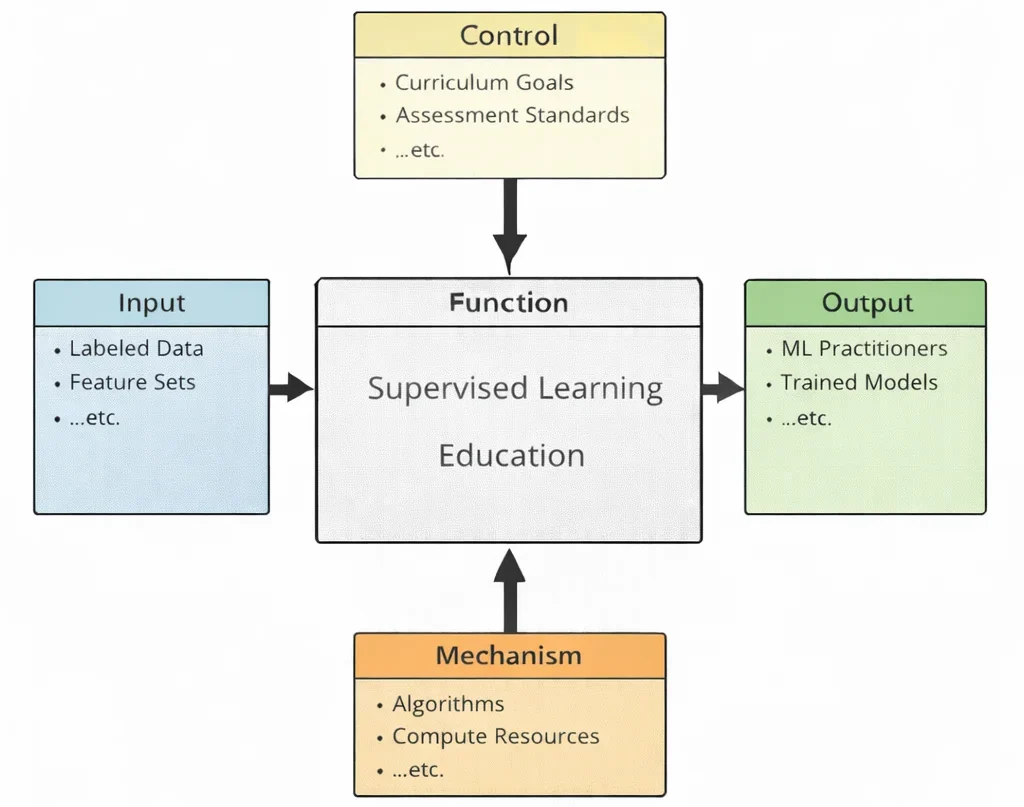
This IDEF0 (Input–Control–Output–Mechanism) diagram presents Supervised Learning Education as a structured learning process. Inputs on the left—labeled data, feature sets, …etc.—represent the core materials of supervised learning, where examples come with “answers” that guide training. Controls at the top—curriculum goals, assessment standards, …etc.—set the learning direction and define how competence is measured, ensuring students learn both method and discipline. The central function, Supervised Learning Education, converts these inputs and controls into practical capability through guided study and hands-on experimentation. Outputs on the right—ML practitioners, trained models, …etc.—represent the intended outcomes: learners who can build, validate, and interpret supervised models, and working models that can make reliable predictions on similar data. Mechanisms at the bottom—algorithms, compute resources, …etc.—provide the enabling infrastructure that makes training and evaluation possible, from standard learning methods to the computing power needed for iterative improvement.
Supervised learning is a core branch of artificial intelligence and machine learning in which models learn from labeled examples to predict outcomes or assign categories. By discovering patterns in historical data, it powers everything from medical diagnosis and credit scoring to demand forecasting and personalized recommendations. In practice it works hand-in-hand with data science & analytics and underpins high-impact applications in computer vision and natural language processing (NLP).
In vision, supervised models label objects and scenes; in language, they classify intent, rate sentiment, or extract entities. These capabilities extend to robotics and autonomous systems, where sensory data must be interpreted in real time. Thanks to cloud computing and flexible cloud deployment models, training can scale from laptops to distributed clusters.
Across the broader STEM landscape, supervised learning supports smart manufacturing & Industry 4.0, optimizes the Internet of Things (IoT), and even contributes to space exploration and satellite technology by enabling reliable onboard classification and prediction.
Supervised learning complements unsupervised learning (which finds structure in unlabeled data) and reinforcement learning (which learns through interaction). Together, these paradigms also strengthen expert systems, where learned components refine rule-based decision making.
Modern results are driven by deep learning, whose multilayer networks learn rich representations from annotated inputs. Looking ahead, ideas from quantum computing—including qubits, superposition, and quantum gates—may unlock new model training and inference strategies.
Beyond research, supervised models quietly run the web: they rank results and ads, filter spam, and power recommenders in internet & web technologies. Within information technology, they detect anomalies for cybersecurity and keep services resilient. For students and practitioners, mastering supervised learning is a foundational step toward building intelligent, reliable systems.

This illustration presents supervised learning as a structured pipeline. A central web of connected nodes suggests a trained model (neural network), while surrounding panels show labeled datasets, performance charts, and prediction outputs. Arrows imply the key idea: the model learns from input–label pairs (examples with correct answers) and then uses that learned mapping to predict labels for new data. The bright, data-rich style reinforces the theme of “learning from examples” across tasks such as classification and regression, where feedback from known labels guides improvement.
Table of Contents
Core Concepts of Supervised Learning
Training with Labeled Data:
The hallmark of supervised learning is the use of data that includes both features and corresponding target labels. For instance, in a dataset of emails, each email might be labeled as either “spam” or “not spam.” By exposing the model to numerous examples, it learns to distinguish subtle patterns that correlate specific features (such as certain keywords, sender addresses, or links) with these labels. Over time, the model refines its decision boundaries, improving its accuracy in predicting unseen cases.
Generalization to New Data:
One of the primary goals of supervised learning is to generalize beyond the training set. A well-trained model can handle data it has never encountered before, making it valuable for real-world applications. The model’s ability to generalize depends on factors like the quantity and diversity of training data, choice of algorithm, and the complexity of the model itself. Balancing these factors helps avoid overfitting (memorizing the training data too closely) or underfitting (failing to learn meaningful patterns).
Iterative Training Process:
Most supervised learning methods involve an iterative training cycle. Initially, the model starts with random or default parameters. As it processes the training data, it makes predictions and compares them to the known labels. By calculating an error measure (e.g., mean squared error for regression problems or accuracy for classification), it adjusts its parameters to reduce this error. Repeating this process many times allows the model to converge on an optimal set of parameters that produce accurate predictions.
Model Evaluation and Validation:
To assess a supervised learning model’s performance, the data is often split into training, validation, and test subsets. The training set teaches the model, the validation set helps tune hyperparameters and prevent overfitting, and the test set serves as a final, unbiased measure of how well the model generalizes. By carefully evaluating results on these sets, developers ensure the model is both accurate and reliable when deployed.
Next, we’ll prepare features safely—avoiding data leakage—so our evaluation remains trustworthy.
Feature Engineering & Leakage-Safe Preprocessing
Put preprocessing steps that learn from data (e.g., scaling, imputation, PCA, target encoding)
inside the train-only fit, then apply to validation/test. In code, use a single pipeline
(e.g., sklearn.Pipeline) so the transforms are fit on the training split only and
reused for val/test. This prevents data leakage—information from validation/test
sneaking into training via preprocessing statistics.
What goes where?
- Fit on train only: Standard/MinMax scaling, robust scaling, imputation, PCA, feature selection, target encoding, text vectorizers (TF-IDF), learned embeddings.
- Safe to precompute globally: Deterministic transforms that don’t “learn” from labels or distribution (e.g., fixed hash buckets, pure regex parsing, unit conversions).
- Be careful with time: compute statistics using only past data; roll your window forward for time-series splits.
High-value engineered features
- Counts/frequencies (per category, user, device) — fit counts on train; smooth to avoid leakage.
- Target/mean encoding — use K-fold or leave-one-out on train; never use raw global target means.
- Text — clean → tokenize → TF-IDF/embeddings; keep vectorizer fitted on train only.
- Images — augmentations only on train; val/test must remain “clean”.
- Time — calendar features (dow, hour, season), lags/rollings with proper causal windows.
Leakage patterns (avoid)
- Scaling/Imputation fit on the full dataset before splitting.
- Target encoding using validation/test targets during fit.
- PCA or feature selection (e.g., SelectKBest) computed on all data.
- Time-series: using future stats (global mean, future rolling windows).
Leakage-safe workflow
- Split first (or use CV folds / time-series splits).
- Build a pipeline: preprocessors + model in one object.
- Fit the pipeline on train (or each CV fold’s train part).
- Evaluate by transforming val/test via the fitted pipeline only.
Tip: With scikit-learn, use Pipeline/ColumnTransformer;
for time-series, prefer TimeSeriesSplit or rolling origin evaluation.
Quick checklist
- All transforms that compute statistics (means, std, medians, vocabularies, PCs, encodings) are fit on train only.
- Target/mean encodings use K-fold scheme on train and never peek at validation/test labels.
- Augmentations: train only. No augmentation on validation/test.
- Time-series: no future leakage; features derived with causal windows.
- One reproducible pipeline used for training, CV, and final inference.
Leakage Smoke Tests (Quick Checks)
Use this lightweight checklist after your main feature-engineering section to catch the most common leakage paths.
- Fit statistics on train only—and re-fit per CV fold (via a Pipeline): scalers, imputers, encoders, PCA, feature selection.
- Time series is causal: split by time; no shuffle across time; windowing never peeks into future rows.
- Target/mean encoding: compute with K-fold/LOO inside the training fold; never use val/test targets.
- Group-aware splits: if samples share an ID (user/patient/device), use
GroupKFoldso groups don’t leak across folds. - Augment only the train split: text/image/audio augmentation must not duplicate or transform validation/test examples.
- Validate transforms re-fit per fold: inspect the pipeline or logs to confirm each fold re-learns preprocessing.
Fast sanity checks
- Shuffle-label test: randomly permute
y; score should drop to chance. If not, something is leaking. - Train↔Val swap: swap splits; a large unexplained jump often signals leakage or distribution shift.
- Feature ablation: remove “suspicious” features (IDs, timestamps close to target) and verify the score behaves sensibly.
CV-safe template (scikit-learn)
from sklearn.pipeline import Pipeline
from sklearn.model_selection import StratifiedKFold, cross_val_score
from sklearn.compose import ColumnTransformer
from sklearn.preprocessing import StandardScaler, OneHotEncoder
from sklearn.linear_model import LogisticRegression

num = ["age","income"]
cat = ["city","channel"]

pre = ColumnTransformer(
    transformers=[
        ("num", StandardScaler(), num),
        ("cat", OneHotEncoder(handle_unknown="ignore"), cat),
    ],
    remainder="drop"
)

pipe = Pipeline([
    ("pre", pre),  # re-fit per fold
    ("clf", LogisticRegression(max_iter=1000))
])

cv = StratifiedKFold(n_splits=5, shuffle=True, random_state=42)
scores = cross_val_score(pipe, X, y, cv=cv, scoring="roc_auc")
print(scores.mean(), scores.std())
Bias–Variance Trade-off & Regularization
In supervised learning, test error reflects three components:
High bias (underfitting) means the model is too simple and misses patterns; high variance (overfitting) means the model memorizes noise and fails to generalize. Good practice seeks a sweet spot that minimizes the sum.
What regularization does
-
L2 / Ridge: shrink coefficients toward 0 (but rarely to exactly 0).\[ \hat{\beta}_{\text{ridge}} = \arg\min_{\beta}\; \frac{1}{n}\sum_{i=1}^n (y_i - x_i^\top \beta)^2 + \lambda \|\beta\|_2^2. \]Stabilizes solutions, lowers variance, improves conditioning.
-
L1 / Lasso: promotes sparsity (feature selection).\[ \hat{\beta}_{\text{lasso}} = \arg\min_{\beta}\; \frac{1}{n}\sum_{i=1}^n (y_i - x_i^\top \beta)^2 + \lambda \|\beta\|_1. \]Helpful when many features are irrelevant.
-
Elastic Net: blend of L1 and L2 for grouped/sparse features.\[ \frac{1}{n}\sum_{i=1}^n (y_i-x_i^\top\beta)^2 + \lambda\left(\alpha\|\beta\|_1 + \frac{1-\alpha}{2}\|\beta\|_2^2\right). \]
- Logistic Regression (classification) uses the same penalties on the negative log-likelihood; choose C = 1/λ in many libraries.
- Early stopping (for boosted trees / neural nets): stop when validation loss stops improving— a powerful, implicit regularizer.
- Data augmentation (esp. vision/text): enlarge training diversity to reduce variance without changing the hypothesis class.
Learning curves & generalization gap
Plot training vs. validation error as data size grows. Parallel curves with a large gap → high variance (try more data/regularization). Both curves high → high bias (try richer features or models).
Practical checklist
- Always standardize inputs before L1/L2; penalties act in feature units.
- Tune λ (or
C=1/λ) via k-fold CV; search on a log scale. - Prefer L1/Elastic-Net when you expect many irrelevant features; prefer L2 when features are correlated and you want stability.
- Watch for data leakage: fit scalers/encoders on the training fold only.
- Report not just accuracy/R² but also the validation curve (metric vs. λ) to show robustness.
When things go wrong
- Exploding coefficients → add/strengthen L2; check multicollinearity.
- Model too sparse under L1 → lower λ or switch to Elastic Net.
- Inconsistent CV scores → increase folds, use stratification, or more data.
Hyperparameter Tuning & Model Selection
Hyperparameters control a model’s capacity and inductive bias. Good tuning improves generalization (not just training accuracy) and ties directly to the bias–variance trade-off. This section shows how to search well, avoid leakage, and make robust choices.
Data splitting for tuning (use the right CV)
- Stratified K-Fold for classification to preserve class ratios on each fold.
- Group K-Fold if samples share an ID (e.g., same user/patient) to prevent group leakage.
- TimeSeriesSplit (expanding window) for temporal data—never shuffle across time.
- Nested CV when you need an unbiased performance estimate: inner loops tune, outer loops evaluate.
Search strategies
- Grid Search: fine scan over a small, well-understood space. Costly in high dimensions.
- Random Search: pick values at random; covers wide spaces efficiently—great default.
- Bayesian/Adaptive: sequentially proposes promising configs (e.g., Optuna, scikit-optimize).
- Early stopping: for boosted trees/NNs, monitor a validation split and stop when metric plateaus.
Practical ranges (quick starting points)
- Logistic Regression (L2):
Cin log-space: {1e-4 … 1e4}. Trypenalty='l2',solver='lbfgs'. - Linear SVM:
Cin {1e-4 … 1e3}. For large sparse text, useLinearSVC. - RBF SVM:
Cin {1e-1 … 1e3},gammain {1e-4 … 1e0} (log-space). - Random Forest:
n_estimators300–800;max_depth6–30;min_samples_leaf1–10; considermax_features√d. - XGBoost/LightGBM/CatBoost:
learning_rate0.01–0.1;n_estimators300–2000 with early-stopping;max_depth4–12;subsample,colsample_bytree0.6–0.9; regularizers (min_child_weight/lambda). - k-NN: k ≈ √n as a start; tune distance metric and feature scaling (critical!).
Choosing the winner (beyond accuracy)
- Pick an objective aligned with the problem: PR-AUC / F1 for imbalanced detection; ROC-AUC for ranking; MAE when large outliers are acceptable, RMSE when they are not.
- Inspect validation curves (score vs. hyperparameter) and learning curves (score vs. data size) to diagnose under/over-fit.
- For classifiers, choose a decision threshold from ROC/PR curves or cost curves—not always 0.5.
- Re-fit the final model on all training data with the chosen hyperparameters; keep a hold-out test for the last check.
Reproducibility & tracking
- Fix
random_state/ seeds; record package versions and data snapshots. - Log experiments (params, CV scores, artifacts) with MLflow/Weights&Biases/Neptune.
- Use the correct CV splitter (Stratified/Group/TimeSeries).
- All transforms live in a Pipeline to avoid leakage.
- Start with Random Search; move to Bayesian if budgets allow.
- For trees/NNs: enable early stopping.
- Decide thresholds and metrics that match business cost/benefit.
- Re-train on full training data; evaluate once on the untouched test set.
Imbalanced Classification, Thresholding & Calibration
Accuracy can be misleading when the positive class is rare. This section shows how to evaluate, tune, and deploy classifiers responsibly when class priors are skewed. You’ll learn which metrics to trust, how to set a decision threshold (not just use 0.5), and how to calibrate predicted probabilities for cost-sensitive decisions.
Why “accuracy” fails & which metrics to use
- Prefer PR-space when positives are rare: Average Precision (AP) / PR-AUC and F1 summarize retrieval performance.
- Balanced Accuracy = (TPR + TNR)/2; robust to skew.
- MCC (Matthews Correlation Coefficient): symmetric, informative with skew and when both classes matter.
- Still plot ROC, but remember that ROC-AUC can look “good” even when precision is poor at operational recall.
- Always report a confusion matrix at the chosen threshold (not just AUCs).
StratifiedKFold so each fold preserves class prior. If the prior in production differs from training, re-estimate it and re-assess thresholds and costs.Tackling class imbalance
- Data-level: downsample the majority; oversample the minority (e.g.,
RandomOverSampler); synthetic generation (SMOTE/ADASYN). Perform resampling inside CV folds to avoid leakage. - Algorithm-level: use
class_weight="balanced"(LogReg, SVM, Tree/Forest, etc.); focal loss (for NNs); tweakmin_samples_leafto avoid memorizing noise. - Evaluation-level: optimize for AP/F1/MCC (or expected cost) rather than raw accuracy; compare PR curves between candidates.
Choosing the decision threshold
Calibrated scores let you pick a threshold that aligns with business cost or desired operating point.
- Metric-based: choose the threshold that maximizes F1, MCC, or balances precision@recalltarget.
- Cost-based: pick
tthat minimizes expected cost:ExpectedCost(t) = CFP·FP(t) + CFN·FN(t). Include prevalence if your validation prior differs from production. - Decision curve analysis: evaluate net benefit across thresholds to show usefulness vs “treat all/none”.
# Pick threshold that maximizes F1 on a validation set
from sklearn.metrics import precision_recall_curve, f1_score
probs = clf.predict_proba(X_val)[:,1]
prec, rec, thr = precision_recall_curve(y_val, probs)
import numpy as np
f1 = (2*prec*rec)/(prec+rec+1e-12)
t_star = thr[np.nanargmax(f1)]
print("Best F1 threshold:", float(t_star))
Probability calibration (for reliable scores)
Many models (trees, SVMs, boosted ensembles) output uncalibrated scores. Calibration maps scores to true probabilities so you can set thresholds by risk/cost and combine models sanely.
- Platt scaling (logistic) is smooth and works well with plenty of data.
- Isotonic regression is non-parametric; great flexibility but needs more data to avoid overfit.
- Use a held-out calibration split or
cv="prefit"withCalibratedClassifierCVafter fitting on train. - Inspect calibration curves and report Brier score.
# Calibrate an already-trained model on a held-out split
from sklearn.calibration import CalibratedClassifierCV, calibration_curve
cal = CalibratedClassifierCV(base_estimator=clf, method="isotonic", cv="prefit")
cal.fit(X_cal, y_cal)       # calibration split
prob_cal = cal.predict_proba(X_val)[:,1]
# now choose threshold on calibrated probabilities (as above)
Quick checklist
- Use Stratified CV and report PR-AUC/AP, MCC, Balanced Accuracy.
- Pick a threshold for production (don’t ship 0.5 by default); document the chosen operating point and rationale.
- Prefer class weights or calibrated thresholding before heavy oversampling.
- When costs differ (e.g., FN ≫ FP), minimize expected cost and present a confusion matrix at that threshold.
- Monitor post-deploy: class prior shift, calibration drift (Brier), and threshold suitability.
Common Techniques in Supervised Learning
Classification:
Classification tasks assign discrete labels to input data. Examples include:
Spam Detection:
Given an email’s content and metadata, a model learns to categorize emails as spam or not spam. After training on labeled examples, it can then accurately classify new incoming emails, alerting users or filtering out unwanted content.
Image Recognition:
In image classification, the model receives images along with labels indicating what each image depicts (e.g., “cat,” “dog,” or “car”). With enough labeled examples, the model can learn to recognize objects, animals, or scenes in new images.
Classification techniques often involve algorithms such as logistic regression, decision trees, random forests, support vector machines (SVMs), and neural networks. Evaluating a classifier’s performance involves metrics like accuracy, precision, recall, and F1-score, each offering unique insights into the model’s strengths and weaknesses.
Regression:
Regression tasks involve predicting continuous numerical values. Examples include:
Predicting Prices:
A model might learn to estimate housing prices based on features such as location, square footage, number of bedrooms, and recent sales data. Once trained, it can forecast the price of a home that the algorithm has never encountered before.
Forecasting Sales:
By examining historical sales data, seasonal trends, and economic indicators, a regression model can anticipate future sales volumes, aiding companies in inventory management and strategic planning.
Common regression algorithms include linear regression, ridge regression, lasso regression, and gradient boosting methods. Metrics like mean squared error (MSE), mean absolute error (MAE), and R² (coefficient of determination) help evaluate how closely the model’s predictions match the actual continuous values.
Model Interpretability & Explainability
Interpretable models build trust, help debug data issues, and support compliant decision-making. Use the tools below to understand global behavior (what the model learned overall) and local behavior (why a single prediction happened).
Global vs. local explanations
- Global: which features matter on average? (permutation importance, SHAP global importance, partial dependence).
- Local: why did this one case get this prediction? (SHAP values, local ICE curves).
Permutation importance (model-agnostic)
Randomly shuffle a feature and see how much performance drops. Works with any estimator and respects your chosen metric (e.g., AP, ROC-AUC, RMSE).
# Global permutation importance on a validation set
from sklearn.inspection import permutation_importance
from sklearn.metrics import average_precision_score
import numpy as np

# y_val_pred = clf.predict_proba(X_val)[:,1]  # for a prob. classifier
print("Val AP:", average_precision_score(y_val, clf.predict_proba(X_val)[:,1]))

imp = permutation_importance(
    clf, X_val, y_val,
    scoring="average_precision", n_repeats=10, random_state=42
)
order = np.argsort(-imp.importances_mean)
for idx in order[:15]:
print(f"{X_val.columns[idx]:24s} mean={imp.importances_mean[idx]:.4f} std={imp.importances_std[idx]:.4f}")Partial Dependence & ICE (how predictions change with a feature)
Partial Dependence (PD) shows the average effect of a feature on the prediction; ICE shows per-row curves. Use both: PD for trend, ICE for heterogeneity.
# Partial Dependence / ICE with scikit-learn
from sklearn.inspection import PartialDependenceDisplay
import matplotlib.pyplot as plt

features_to_plot = ["age", "income"]
PartialDependenceDisplay.from_estimator(
    clf, X_val, features_to_plot, kind="both", # "average" (PD), "individual" (ICE), or "both"
    grid_resolution=40
)
plt.tight_layout(); plt.show()SHAP values (local & global)
SHAP gives per-feature contributions for each prediction, and aggregates to global importance. TreeExplainer is fast for tree-based models; KernelExplainer works for any model (but can be slow).
# SHAP for a tree-based model (e.g., LightGBM / XGBoost / RandomForest)
import shap
explainer = shap.TreeExplainer(clf)          # clf is a fitted tree-based model
shap_values = explainer.shap_values(X_val)   # classification: array; regression: matrix

# Global importance (bar) and summary plot (beeswarm)
shap.summary_plot(shap_values, X_val, plot_type="bar")     # global ranking
shap.summary_plot(shap_values, X_val)                      # distribution & direction

# Local explanation for a single case
i = 0
shap.force_plot(explainer.expected_value, shap_values[i], X_val.iloc[i,:])Checklist
- Explain on validation or OOF data, not the training fold used to fit.
- Use permutation importance as a quick, metric-aware global signal; confirm with SHAP.
- Plot PD + ICE to verify sensible monotonic or saturating behaviors.
- Watch out for correlated features; group them or perform conditional PD/accumulated local effects if available.
- Document findings (which features drive decisions, stability across folds) and attach confusion matrix at the chosen threshold for the business audience.
Production Monitoring & Drift
After deployment, models need guardrails. Monitor data quality, distribution drift, calibration, and business KPIs; alert when they breach thresholds; and retrain on a schedule or when drift persists.
What to watch
- Data quality: schema, missing/invalid rates, range checks, category explosions.
- Data drift (covariate shift): input features change vs. training (PSI, KS, JS/KL).
- Label/target drift: base rate changes (if labels available with delay).
- Concept drift: relationship between X and y changes (online error / rolling KPI rises).
- Calibration drift: predicted probabilities no longer match observed rates (ECE/Brier).
- Business KPIs: precision@k, recall@threshold, conversion, cost.
Minimal logging contract
Log every prediction (or a sample) with enough fields to recompute metrics and audit decisions:
{
  "ts":"2025-01-10T13:15:20Z",
  "model":"fraud_v12",
  "version":"12.3.1",
  "request_id":"6f9a-...",
  "features":{"age":43,"country":"SG","amount":129.5,...},
  "score":0.8123,
  "threshold":0.72,
  "decision":"flag",
  "ground_truth": null          // fill later when available
}
Quick drift/eval utilities (scikit-learn compatible)
# --- Population Stability Index (PSI) for one feature ---
import numpy as np

def psi(expected, actual, bins=10):
    e, edges = np.histogram(expected, bins=bins)
    a, _      = np.histogram(actual,   bins=edges)
    e = e / (e.sum() + 1e-12)
    a = a / (a.sum() + 1e-12)
    e = np.clip(e, 1e-6, None)
    a = np.clip(a, 1e-6, None)
    return np.sum((a - e) * np.log(a / e))

# --- KS test for continuous feature drift ---
from scipy.stats import ks_2samp
def ks_drift(expected, actual):
    stat, p = ks_2samp(expected, actual)
    return stat, p    # alert when stat > 0.1 (rule-of-thumb) and p < 0.01

# --- Expected Calibration Error (ECE) for binary probs ---
def ece(probs, labels, n_bins=15):
    bins = np.linspace(0,1,n_bins+1)
    idx = np.digitize(probs, bins) - 1
    ece = 0.0
    for b in range(n_bins):
        sel = idx == b
        if sel.any():
            conf = probs[sel].mean()
            acc  = labels[sel].mean()
            ece += probs[sel].size / probs.size * abs(acc - conf)
    return ece

# Example usage:
# psi_val = psi(train_df["amount"], prod_df["amount"])
# ks_stat, ks_p = ks_drift(train_df["age"], prod_df["age"])
# ece_val = ece(probs=val_pred_proba, labels=val_labels)
Typical alert thresholds (starting points)
- PSI: < 0.1 = small; 0.1–0.25 = moderate (investigate); > 0.25 = high (alert).
- KS: stat > 0.1 with p < 0.01 → drift likely.
- Calibration:
ECE> 0.05 on the main slice or large increase vs. baseline. - KPIs: sustained drop > X% for Y days (e.g., precision@k down 20% for 3 days).
Rolling backtests & dashboards
- Compute daily metrics: PSI (top features), KS/ECE, AUROC/PR-AUC (if labels available), precision/recall at your operating threshold(s).
- Trend them in a dashboard (Grafana/Looker/Metabase) with SLO lines and alert rules.
- Slice by segment (country, device, channel) to catch localized drift early.
Retraining policy (example)
- Time-based: retrain monthly; keep last N models for safe rollback.
- Event-based: if >= 2 high-drift signals (e.g., PSI>0.25 on 3 key features) persist for 5 days, start expedited retraining.
- Shadow validation: score new model in shadow for 1–2 weeks; promote if it beats current on held-out labels and live KPIs.
Data quality smoke tests (fast)
- Schema & type checks; categorical cardinality caps; numeric range/percentile guards.
- Missing value rate changes > X% vs. baseline → alert.
- Feature store/ETL version pinning; log provenance (
dataset_version,feature_view).
Summary checklist
- Log scores, features (or hashes for PII safety), decisions, and delayed labels.
- Track PSI/KS for top features, ECE for calibration, and business KPIs daily.
- Set SLOs + alerts; use rolling windows and per-segment views.
- Adopt a clear retraining & shadow-promotion policy; keep rollback ready.
Fairness & Responsible ML
Assess performance across sensitive groups and constrain harm. Measure, monitor, and (when needed) mitigate disparities while documenting trade-offs and approvals.
Key fairness notions (binary classification)
- Demographic Parity (selection rate parity): \( P(\hat{Y}=1 \mid A=a) \) similar across groups.
- Equal Opportunity: true positive rate parity \( \text{TPR}(\,A=a\,) \) across groups.
- Equalized Odds: parity of both TPR and FPR across groups.
- Calibration within groups: predicted probabilities reflect observed frequencies per group.
- Disparate Impact Ratio: \( \min_a \frac{\Pr(\hat{Y}=1 \mid A=a)}{\max_{a'} \Pr(\hat{Y}=1 \mid A=a')} \) (rule-of-thumb alert if < 0.8).
Audit checklist
- Define sensitive attributes (e.g., gender, age band, region); ensure lawful use and consent.
- Report per-group: support (n), AUROC/PR-AUC, TPR/FPR/TNR, Precision/Recall, calibration (ECE/Brier), selection rate.
- Compute gap metrics: max-min differences and ratios (e.g., disparate impact).
- Review slices (intersectional groups) with minimum sample thresholds to reduce noise.
- Record threshold policy (single vs. group-specific) and the rationale.
Mitigation options
- Pre-processing: reweighing/oversampling; privacy-safe transformations; leakage-safe encodings.
- In-processing: add constraints/penalties (e.g., fairness-regularized loss); adversarial debiasing.
- Post-processing: adjust decision thresholds per group to meet a target (e.g., equal opportunity), with impact analysis.
Per-group metrics (quick Python)
import numpy as np
import pandas as pd
from sklearn.metrics import roc_auc_score, precision_recall_fscore_support

def group_report(df, y_true, y_score, group_col, threshold=0.5):
    out = []
    for g, sub in df.groupby(group_col):
        y  = sub[y_true].values
        s  = sub[y_score].values
        yh = (s >= threshold).astype(int)
        tp = ((yh==1) & (y==1)).sum()
        fp = ((yh==1) & (y==0)).sum()
        tn = ((yh==0) & (y==0)).sum()
        fn = ((yh==0) & (y==1)).sum()
        tpr = tp / (tp+fn+1e-9)
        fpr = fp / (fp+tn+1e-9)
        prec, rec, f1, _ = precision_recall_fscore_support(y, yh, average='binary', zero_division=0)
        auroc = roc_auc_score(y, s) if len(np.unique(y))==2 else np.nan
        sel_rate = yh.mean()
        out.append(dict(group=g, n=len(sub), auroc=auroc, tpr=tpr, fpr=fpr,
                        precision=prec, recall=rec, f1=f1, select_rate=sel_rate))
    rep = pd.DataFrame(out)
    # Disparate impact ratio (selection rates)
    di = rep['select_rate'].min() / (rep['select_rate'].max()+1e-9)
    return rep, di

# Example:
# rep, di = group_report(df, y_true="label", y_score="score", group_col="gender", threshold=0.6)
# print(rep); print("Disparate impact ratio:", round(di, 3))
Post-processing thresholds (equal opportunity target)
Choose per-group thresholds \( \tau_a \) to align TPRs while tracking precision & cost. Start with a simple line search per group to hit a target TPR.
def threshold_for_tpr(scores, labels, target_tpr):
    # scores, labels are 1-D arrays for a single group
    thresh_candidates = np.quantile(scores, np.linspace(0.0, 1.0, 101))
    best = thresh_candidates[0]; best_gap = 1e9
    for t in thresh_candidates:
      pred = (scores >= t).astype(int)
      tp = ((pred==1) & (labels==1)).sum()
      fn = ((pred==0) & (labels==1)).sum()
      tpr = tp / (tp+fn+1e-9)
      if abs(tpr - target_tpr) < best_gap:
          best, best_gap = t, abs(tpr - target_tpr)
    return float(best)
Governance & documentation
- Model card: intended use, data sources, known limitations, fairness metrics & decisions.
- Approval trail: who signed off, on what metrics/thresholds, and when.
- Monitoring: track fairness metrics over time (same cadence as accuracy & drift dashboards).
Data Privacy & PII Handling
Protect personal data end-to-end: collect only what you need, minimize exposure in ML pipelines, and enforce access, retention, and audit controls. The patterns below are implementation-agnostic and work with common MLOps stacks.
PII taxonomy & tagging
Label columns with classification and handling rules so pipelines can enforce them automatically.
| Field | Examples | Class | Default Handling |
|---|---|---|---|
| Direct identifiers | Name, email, phone, national ID | Sensitive | Do not store raw; tokenize or HMAC-hash with secret key; restrict access |
| Quasi-identifiers | DoB, postcode, device ID, IP | Restricted | Generalize/bucket; consider hashing; apply retention limits |
| Free-text | Support notes, forms | Unknown | Run PII redaction before storage; avoid in feature store |
| Labels/targets | Default flag, diagnosis | Restricted | Access-controlled; document purpose & legal basis |
| Aggregates/features | Counts, rates, embeddings | Low | Keep derived only; avoid carrying raw PII downstream |
Minimize, purpose-limit & retention
- Collect only attributes needed for the stated ML purpose; document lawful basis.
- Derive features then drop raw PII (e.g., keep “domain of email”, not full address).
- Retention: define per-field days to live; auto-purge expired partitions/snapshots.
De-identification techniques
- Masking/truncation: e.g.,
email → e***@example.com. - Deterministic tokenization (reversible via vault) for join keys when lookups are required.
- Hashing with secret salt (HMAC) for pseudonymous joins; not reversible.
- Generalization: bucket ages, round timestamps, coarsen location granularity.
- k-anonymity / l-diversity: ensure quasi-identifier groups have ≥k rows and diverse sensitive values.
HMAC pseudonymization (Python)
import hmac, hashlib, base64, os

# Load a secret key from KMS or env (rotate periodically)
SECRET = os.environ["PII_HMAC_KEY"].encode("utf-8")

def pseudonymize(value: str) -> str:
    if value is None or value == "":
        return ""
    digest = hmac.new(SECRET, value.encode("utf-8"), hashlib.sha256).digest()
    # short, URL-safe token (non-reversible)
    return base64.urlsafe_b64encode(digest).decode("utf-8")[:32]

# Example: replace direct identifiers at ingestion time
# df["email_tok"] = df["email"].apply(pseudonymize); del df["email"]
Secrets & key management
- Keep salts/keys in a KMS/secret manager; never hard-code in notebooks or configs.
- Rotate regularly and version tokens if you need revocation.
- Encrypt in transit (TLS) and at rest (disk/object store; column-level if supported).
Access control & auditing
- RBAC/ABAC with least privilege; separate roles for ingestion, feature engineering, training, serving.
- Column/row-level security and masked views for restricted fields.
- Audit logs: who accessed which fields and when; include purpose and ticket/approval id.
- Redact PII in app and pipeline logs; never dump raw data in error messages or exceptions.
Safe ML workflow pattern
- Ingest to a red zone (restricted), tokenize/hash direct IDs, then move derived features to a green zone (feature store).
- Join training data on tokens, not raw IDs. Keep the token↔raw lookup only in a secure vault if business needs require reidentification.
- Validate outbound datasets (reports/exports) with an egress rule: no columns tagged as
PII:direct.
Schema contract with tags (example)
{
  "field": "email",
  "tags": ["PII:direct","restricted"],
  "handling": {"strategy":"hmac_sha256","salt_key":"kms:pii_salt_v3"},
  "retention_days": 90,
  "access_role": "pii_readers",
  "purpose": "fraud_detection"
}
{
  "field": "age",
  "tags": ["quasi","restricted"],
  "handling": {"strategy":"bucket","bins":[0,18,25,35,45,55,65,120]},
  "retention_days": 730,
  "access_role": "analyst",
  "purpose": "risk_scoring"
}
Data-subject rights (DSRs)
- Support delete/rectify/export requests; keep token maps so deletions can propagate.
- Log DSR actions with timestamps and affected datasets/models.
Practical Considerations:
Feature Selection and Engineering:
Choosing the right features is critical. Irrelevant or redundant features can confuse the model, while well-crafted features can significantly improve accuracy. Students and practitioners often experiment with feature scaling, dimensionality reduction, or domain-specific transformations to enhance model performance.
Handling Imbalanced Classes and Missing Data:
Real-world datasets are rarely perfect. Models must handle issues such as imbalanced classes (e.g., far fewer “spam” emails than “not spam”), missing values, or noisy data. Techniques like oversampling minority classes, imputing missing data, or cleaning outliers help create more robust models.
Ethical and Fairness Considerations:
Since supervised learning models rely on historical data, they can inadvertently perpetuate biases if the training data is not carefully vetted. Ensuring diverse and representative training sets, as well as applying fairness metrics and bias mitigation strategies, is essential for building ethical machine learning solutions.
Evaluation & Metrics (Supervised Learning)
Choose metrics that match the task and business costs. Always report results with stratified cross-validation and avoid leakage (fit scalers/encoders only on the train fold).
Classification
With positives as class 1 and confusion matrix counts \((TP, FP, FN, TN)\):
\[ \text{Accuracy}=\frac{TP+TN}{TP+FP+FN+TN},\qquad \text{BalancedAcc}=\frac{1}{2}\big(\text{TPR}+\text{TNR}\big). \] \[ \text{Precision}=\frac{TP}{TP+FP},\quad \text{Recall}=\frac{TP}{TP+FN},\quad F_1=\frac{2\,\text{Precision}\cdot\text{Recall}}{\text{Precision}+\text{Recall}}. \]
- ROC–AUC: threshold-free separability; can look optimistic under heavy class skew.
- PR–AUC: emphasizes the positive class; preferred for rare events.
- MCC (Matthews Corr. Coef.): \[ \mathrm{MCC}= \frac{TP\cdot TN-FP\cdot FN} {\sqrt{(TP+FP)(TP+FN)(TN+FP)(TN+FN)}}. \] Stable under imbalance.
- Log Loss (cross-entropy) and Brier score assess probability quality.
Choosing a Threshold
For a calibrated probability \(p(x)=P(y=1\mid x)\), the default \(0.5\) rarely matches costs. If false positives and false negatives have costs \(c_{FP}, c_{FN}\) and \(c_{TP}=c_{TN}=0\), a Bayes-optimal threshold is
\[ \tau^*=\frac{c_{FP}}{c_{FP}+c_{FN}}. \]
Sweep \(\tau\) on a validation set to maximize \(F_\beta\) (recall-weighted), PR–AUC, or to minimize expected cost \(\text{Cost}(\tau)=c_{FP}P(\hat y_\tau=1,y=0)+c_{FN}P(\hat y_\tau=0,y=1)\).
Calibration (for Probabilities)
- Platt scaling (logistic on scores), isotonic regression (non-parametric), and temperature scaling (for neural nets).
-
Report Brier and ECE (Expected Calibration Error):
\[ \mathrm{Brier}=\frac{1}{n}\sum_{i=1}^{n}(p_i-y_i)^2 \]\[ \mathrm{ECE}=\sum_{b=1}^{B}\frac{n_b}{n}\,\left|\mathrm{acc}(b)-\mathrm{conf}(b)\right| \]
Regression
For targets \(y_i\) and predictions \(\hat y_i\):
\[ \text{MAE}=\frac{1}{n}\sum_{i=1}^n|y_i-\hat y_i|,\quad \text{MSE}=\frac{1}{n}\sum_{i=1}^n(y_i-\hat y_i)^2,\quad \text{RMSE}=\sqrt{\text{MSE}}. \] \[ R^2=1-\frac{\sum_{i}(y_i-\hat y_i)^2}{\sum_{i}(y_i-\bar y)^2}. \]
- Use MAE for robustness to outliers, RMSE when large errors matter more.
- Check residual plots for heteroskedasticity and bias; report prediction intervals if relevant.
Reporting Best Practices
- Use stratified splits for classification; maintain time order for time-series (rolling CV).
- Always compute metrics on a held-out validation/test set untouched by training or preprocessing.
- Provide learning curves (score vs. train size) to diagnose under/overfitting.
Imbalanced Classification, Thresholding & Calibration
Many real problems (fraud, disease, rare failures) have far fewer positives than negatives. Accuracy can be misleading; a model that predicts “negative” for everyone may score 99.9% accuracy yet be useless. Use metrics and techniques that respect class skew and the costs of mistakes.
Confusion Matrix & Core Metrics
With positives as class 1:
\[ \text{Precision}=\frac{TP}{TP+FP},\qquad \text{Recall}=\frac{TP}{TP+FN},\qquad F_1=\frac{2\,\text{Precision}\cdot\text{Recall}}{\text{Precision}+\text{Recall}}. \]
- ROC–AUC is threshold-free but can look optimistic under heavy skew.
- PR–AUC focuses on the positive class and is often more informative when positives are rare.
- Balanced Accuracy = \((\text{TPR}+\text{TNR})/2\) prevents the majority class from dominating.
Choosing a Decision Threshold
If the model outputs a probability \(p(x)=P(y=1\mid x)\), the default threshold \(0.5\) is rarely optimal. When false positives and false negatives have different costs (\(c_{FP}, c_{FN}\)) and we assume \(c_{TP}=c_{TN}=0\), the Bayes-optimal threshold is
\[ \tau^* \;=\; \frac{c_{FP}}{c_{FP}+c_{FN}}. \]
Predict \(1\) when \(p(x) \ge \tau^*\). If you have an operating budget, regulation, or service-level constraint, you can sweep \(\tau\) and select the point that maximizes \(F_\beta\) (recall-weighted), PR–AUC on a validation set, or minimizes expected cost:
\[ \text{Cost}(\tau) \;=\; c_{FP}\,P(\hat y_\tau=1,y=0) + c_{FN}\,P(\hat y_\tau=0,y=1). \]
Strategies for Imbalanced Data
- Class weighting: give a larger loss weight to the minority class (e.g., \(w_1 \propto 1/\pi_1\)).
- Resampling: under-sample majorities or over-sample minorities (e.g., SMOTE/ADASYN) within each CV fold to avoid leakage.
- Focal loss (for neural nets): \[ \text{FL}(p_t)=-\,\alpha(1-p_t)^\gamma\log(p_t), \] which down-weights easy examples and focuses learning on hard, minority errors.
- Ensembles: balanced random forests or gradient boosting with
scale_pos_weight/ class weights.
Probability Calibration
Many models output scores that are not true probabilities. Calibrated probabilities let you set thresholds by economics, combine models, and communicate risk.
- Platt scaling: fit a logistic regression on validation logits/scores.
- Isotonic regression: a monotonic non-parametric mapping; often better with lots of data.
- Temperature scaling (for neural nets): scale logits by a single parameter \(T\).
Two useful calibration metrics:
\[ \mathrm{Brier\ Score}=\frac{1}{n}\sum_{i=1}^{n}(p_i-y_i)^2 \] \[ \mathrm{ECE}=\sum_{b=1}^{B}\frac{n_b}{n}\,\left|\mathrm{acc}(b)-\mathrm{conf}(b)\right| \]
Practical Checklist
- Use stratified train/validation splits; compute PR–AUC and calibration, not accuracy alone.
- Apply resampling/weights inside each CV fold; never before the split (avoids leakage).
- Calibrate on a clean validation set (post-training), then pick \(\tau\) from costs or \(F_\beta\) targets.
- Report a Decision Curve: expected net benefit over thresholds, to show real-world utility.
Time-Series with Supervised Learning (forecasting & leakage-safe CV)
Many forecasting problems can be tackled with ordinary supervised models once you turn the series into lagged features + future targets—but you must keep splits and preprocessing causal to avoid leakage.
Problem setups
- Horizon h: one-step ahead (h=1) or multi-step (h∈{1..H}).
- Prediction strategies: recursive (feed own predictions forward), direct (one model per horizon), MIMO (multi-output for all horizons).
- Exogenous (exog) features: promotions, prices, weather, calendar, etc.
- Multiple entities: series ID (store/product/sensor). Use grouped splits.
Leakage-safe CV & splits
- No shuffling; use expanding-window or rolling-origin evaluation.
- Fit scalers/encoders/feature builders on the train fold only; refit every fold.
- For many entities, split by time within each group or reserve last time slice per group.
- Keep the same horizon gap between train end and validation start.
Expanding-window validation (concept)
Feature cookbook (safe & useful)
- Lags: \(y_{t-1}, y_{t-2}, \dots\) (per entity).
- Rolling stats: mean/median/std/min/max; rolling counts; exponentially-weighted means.
- Differences & growth: \(\Delta y_t = y_t - y_{t-1}\), % change, log-diff.
- Calendar: day-of-week/holiday/season flags; pay-day; month-end; hour-of-day.
- Events & promos: binary flags and intensities (shifted forward if they are decided in advance).
- Exogenous regressors: weather, prices, macro series—use their known-in-advance values only.
Metrics that matter
- MAE/MAPE: MAE is robust and unit-interpretable; MAPE fails near zero.
- sMAPE: \( \displaystyle \mathrm{sMAPE}= \frac{1}{n}\sum \frac{2|y-\hat y|}{|y|+|\hat y|} \).
- Quantile (pinball) loss for P50/P90: enables prediction intervals and service-level planning.
- Weighted metrics (by volume/revenue) for portfolio forecasts.
Baselines & model choices
- Naïve / Seasonal-naïve: yesterday or last-season value—always include as a baseline.
- Classical + regression: STL/seasonal dummies + linear/GBDT on lags & exog.
- Tabular boosters: LightGBM/CatBoost/XGBoost with careful lags & group IDs.
- When to go deep: long horizons, many correlated series, complex exog (then consider TFT/N-Beats).
Production & backtesting
- Backtest over multiple cut-dates (rolling origin); compare against naïve.
- Recreate the known-at-forecast-time feature set in production (feature-time travel checks).
- Log forecasts, features, horizon, and model version for auditability.
- Reconcile hierarchical forecasts (store→region→country) if needed.
Leakage-safe template (scikit-learn)
# Rolling-origin CV with a Pipeline that refits preprocessing per fold
from sklearn.model_selection import TimeSeriesSplit, cross_val_score
from sklearn.compose import ColumnTransformer
from sklearn.preprocessing import StandardScaler, OneHotEncoder
from sklearn.pipeline import Pipeline
from sklearn.linear_model import Ridge

num = ["lag_1","lag_7","roll7_mean","price"]
cat = ["store_id","dow","is_holiday"]

pre = ColumnTransformer(
    transformers=[
        ("num", StandardScaler(), num),
        ("cat", OneHotEncoder(handle_unknown="ignore"), cat),
    ],
    remainder="drop"
)

pipe = Pipeline([
    ("pre", pre),         # refit inside every fold
    ("clf", Ridge(alpha=1.0)),
])

tscv = TimeSeriesSplit(n_splits=5, gap=1, test_size=28)  # keep a horizon gap
scores = cross_val_score(pipe, X, y, cv=tscv, scoring="neg_mean_absolute_error")
print("MAE per fold:", -scores)
Quick checklist
- ✅ Splits are time-ordered (no shuffle); transforms refit per fold.
- ✅ Features use only information available at forecast time.
- ✅ Baseline (seasonal-naïve) is beaten across multiple cut-dates.
- ✅ Report MAE/quantile errors by horizon and by entity (store/product).
Beyond the Basics
As students and developers gain confidence with supervised learning, they can explore more advanced topics such as ensemble methods (e.g., combining multiple models to improve performance), transfer learning (reusing models trained on related tasks), and active learning (efficiently querying labels for new data to reduce labeling costs).
Why Study Supervised Learning
Building the Foundation for Predictive Artificial Intelligence
Learning Key Algorithms and Their Applications
Developing Practical Skills in Data Preparation and Model Evaluation
Understanding Limitations and Ethical Considerations
Preparing for Further Study and Diverse Career Paths
Key Terms (Supervised Learning)
A compact glossary of concepts referenced throughout this page. Definitions are short and practical; where relevant, we include a small formula or rule-of-thumb.
- Supervised Learning
- Learn a mapping from features
Xto label/targetyusing labeled data. - Instance / Example
- One row of data (features + label).
- Feature (Predictor)
- An input variable used by the model (numeric, categorical, text-derived, etc.).
- Label / Target
- The outcome the model tries to predict (class or numeric value).
- Train / Validation / Test Split
- Train fits parameters; validation selects hyperparameters/thresholds; test is held out for final, unbiased evaluation.
- Cross-Validation (CV)
- Repeated splitting of data to estimate generalization. Use Stratified for classification, GroupKFold for grouped entities, TimeSeriesSplit for temporal data.
- Pipeline
- A single object chaining preprocessing and model so transforms are fit on train only and reused on val/test (prevents leakage).
- Data Leakage
- Information from validation/test “sneaks” into training via preprocessing or features; causes overly optimistic metrics.
- Feature Engineering
- Transformations that create informative inputs (scaling, encodings, counts, lags, text vectors). Fit learned transforms on train only.
- One-Hot Encoding
- Binary columns for each category; good for low cardinality.
- Target / Mean Encoding
- Replace categories with smoothed target means; compute out-of-fold on train; never peek at validation/test labels.
- Standardization / Normalization
- Scale features (e.g., z-score) to help linear models/NNs; trees are scale-invariant.
- Parameters vs. Hyperparameters
- Parameters are learned from data (weights). Hyperparameters you set (e.g., depth, C, learning rate).
- Regularization (L1/L2)
- Penalties that curb overfitting. L1 (lasso) encourages sparsity; L2 (ridge) shrinks weights smoothly; Elastic Net mixes both.
- Bias–Variance Trade-off
- Bias (underfit) vs. variance (overfit). Adjust capacity/regularization to find the sweet spot.
- Overfitting / Underfitting
- Overfit: great on train, weak on val/test. Underfit: weak everywhere. Check learning/validation curves.
- Early Stopping
- Stop training when validation metric stops improving (boosted trees, neural nets).
- Class Imbalance
- One class is rare. Prefer PR-AUC/AP, F1, MCC; use class weights, calibrated thresholds, or careful resampling.
- Decision Threshold
- Probability cut-off for classification; choose using costs or metric maximization—don’t default to 0.5.
- Calibration
- Make predicted probabilities reflect true frequencies (Platt scaling, isotonic). Track Brier score / ECE.
- Confusion Matrix
- Counts of TP/FP/FN/TN at a chosen threshold; always show alongside AUCs.
- Precision / Recall / F1
Precision=TP/(TP+FP),Recall=TP/(TP+FN),F1=2·P·R/(P+R).- ROC-AUC / PR-AUC
- ROC-AUC: threshold-free separability; may be optimistic under skew. PR-AUC/AP: better when positives are rare.
- MCC (Matthews Corr. Coef.)
- Balanced correlation-like metric robust to class skew; good single-number summary.
- Baseline
- Simple comparator (majority class, mean, or linear model). A real model must beat this honestly.
- Permutation Importance
- Global, model-agnostic feature importance: shuffle a feature and see metric drop.
- PD / ICE
- Partial Dependence (average effect) and Individual Conditional Expectation (per-row curves) to understand how predictions change with a feature.
- SHAP Values
- Local feature contributions that also aggregate to global importance; fast for tree models.
- Expected Cost
- Evaluate with costs:
Cost(t)=C_FP·FP(t)+C_FN·FN(t); pick threshold/operating point that minimizes it. - Resampling
- Over/undersampling or synthetic examples (SMOTE/ADASYN) used inside CV folds to avoid leakage.
- Class Weights
- Give the minority class higher loss weight to balance gradients (LogReg, SVM, Trees/GBDT).
- HPO (Hyperparameter Optimization)
- Grid/Random search or Bayesian methods to find good hyperparameters under proper CV.
- Drift
- Data (covariate) drift: inputs shift; label drift: base rate changes; concept drift: the relationship between X and y changes.
- PSI / KS
- Population Stability Index and Kolmogorov–Smirnov tests to detect distribution drift between training and production.
- Brier Score / ECE
- Calibration metrics: lower is better. Use with reliability plots.
- Model Card
- Short document describing intended use, data, metrics, limitations, thresholds, and governance status.
- Fairness Criteria
- Demographic Parity, Equal Opportunity, Equalized Odds, Calibration within groups; measure per-group gaps and ratios.
- PII
- Personally Identifiable Information. Minimize, pseudonymize (HMAC/hash), restrict access, and set retention.
- Monitoring
- Ongoing checks post-deployment: drift, calibration, KPIs, per-group metrics, alerting, retrain policy.
- Shadow Deployment
- Run a new model in parallel without affecting users; compare to current model on live traffic.
- Rollback
- Ability to revert to a prior version quickly if metrics or KPIs regress.
- Reproducibility
- Fixed seeds, versioned data/code, and logged experiments to replicate results consistently.
Supervised Learning: Frequently Asked Questions
How do I choose the right evaluation metric for my problem?
Start from the business cost: which mistake is more painful—false positives or false negatives? For rare positives (fraud, disease), accuracy and ROC-AUC can be misleading; prefer PR-AUC or F1, and always show a confusion matrix at the operating threshold. For ranking tasks, ROC-AUC is fine; for calibrated decisions, monitor log loss and Brier score as well.
For regression, use MAE when robustness to outliers matters, and RMSE when large errors should be penalized more. Always compare across stratified or time-respecting validation splits to avoid optimistic results.
Should I scale features for tree-based models?
Decision trees and tree ensembles (Random Forest, Gradient Boosting) are invariant to monotonic scaling—so standardization rarely changes their split logic. However, scaling still helps when you mix models (e.g., comparing to linear/SVM/NN baselines) and for distance-based methods (k-NN) or neural nets.
Focus tree preprocessing on leakage-safe imputation, missing-value indicators, sensible binning (if needed), and robust handling of high-cardinality categoricals (e.g., target encoding out-of-fold).
What is data leakage and how do I prevent it?
Leakage happens when information from validation/test “sneaks” into training (e.g., fitting scalers/encoders/PCA on the whole dataset, or using future data in time series). It inflates metrics and collapses in production.
Prevent it by splitting early, then fitting all learned transforms inside the training fold only via a single Pipeline. For time series, use causal windows and TimeSeriesSplit. For target/mean encoding, compute values out-of-fold on the training split and never peek at validation/test labels.
How do I set the decision threshold for a classifier?
Don’t ship the default 0.5. On a validation set, sweep thresholds and pick one that optimizes the metric you care about (F1, MCC, precision@target recall) or minimizes expected cost given FP/FN costs. If you deploy calibrated probabilities, re-evaluate thresholds when class prevalence shifts in production.
Document the chosen operating point, show the associated confusion matrix, and monitor post-deploy to catch drift that requires re-tuning.
What works best for imbalanced datasets?
First, measure with PR-AUC/AP and F1 (or cost). Enable class_weight="balanced" for linear/SVM/tree models and consider focal loss for neural nets. If resampling, do it inside CV folds (e.g., RandomOverSampler/SMOTE) to avoid leakage.
Calibrated probabilities plus a cost-aware threshold often beat aggressive resampling. Always compare PR curves between candidates rather than relying solely on accuracy.
How should I split data for fair evaluation?
Use Stratified K-Fold for classification to preserve class ratios, GroupKFold when rows share an entity (users/patients), and TimeSeriesSplit with an expanding window for temporal data. Consider nested CV when you need an unbiased performance estimate after hyperparameter tuning.
Always fit preprocessing inside each training fold; evaluate on the corresponding validation fold to keep estimates honest.
Do I need probability calibration?
If your downstream decision uses probabilities (e.g., risk pricing, triage), yes—check calibration. Tree ensembles and SVMs are often miscalibrated out of the box. Use Platt scaling (logistic) or isotonic regression on a held-out calibration split, then re-select your decision threshold using calibrated scores.
Monitor Brier score and ECE in production; recalibrate when they drift, even if you keep the same model weights.
What’s the simplest reliable baseline to start with?
A leakage-safe pipeline with imputation + (optional) scaling + a regularized linear model (logistic regression for classification, ridge/elastic net for regression). Report stratified/time-aware CV metrics and a confusion matrix at the chosen threshold.
Only move to more complex models if they deliver a clear, validated gain on the same evaluation protocol.
How can I interpret model predictions?
For global insight, use permutation importance (metric-aware, model-agnostic) and Partial Dependence (PD). For local reasoning, use SHAP or ICE curves. Compute explanations on validation or out-of-fold data, not on the training fold that fit the model.
When domain rules apply (e.g., risk should not decrease as debt increases), consider monotonic constraints in boosted trees and verify with PD/ICE plots.
How do I monitor a supervised model in production?
Log predictions, features (or hashed), decisions, thresholds, and delayed labels. Track data drift (PSI/KS), calibration (Brier/ECE), and business KPIs daily; set alerts when thresholds are breached.
Adopt a retraining policy (time-based + event-based), and validate new models in shadow before promotion.
How do I handle PII and compliance in ML pipelines?
Minimize collection, pseudonymize early (HMAC/hashed tokens), and restrict access by role. Drop raw identifiers after deriving features, set retention limits per field, and audit access.
Coordinate with legal/compliance for sensitive attributes and fairness auditing; document decisions in a model card.
Supervised Learning: Conclusion
Supervised learning enables models to generalize from labeled examples and make dependable predictions on unseen data. It drives real products and decisions across domains—fraud detection, medical triage, vision and language tasks, demand forecasting, and control—making it a cornerstone of modern AI.
Strong results come from getting the fundamentals right: high-quality labels, leakage-safe preprocessing, honest validation (CV/holdout), fit-for-purpose metrics and calibration, and careful regularization and tuning. With these in place, simple baselines become powerful; complex models add value only when they truly improve generalization.
As deep learning, responsible AI, and MLOps mature, supervised learning will keep evolving. Mastering it gives a durable foundation for building trustworthy systems today and for exploring adjacent areas—semi-/self-supervised learning and reinforcement learning—tomorrow.
Closing Summary & What to Do Next
Supervised learning succeeds when your pipeline is leakage-safe, tuned with the right cross-validation, measured with task-appropriate metrics, and monitored after deployment. Use the steps and links below to move from concepts to a working, trustworthy system.
Action plan (hands-on)
- Start simple: baseline with a regularized linear model and a leakage-safe Pipeline.
- Tune properly: use Stratified/Group/TimeSeries CV; begin with Random Search, then refine.
- Pick the right metric: PR-AUC/F1 for rare positives; MAE/RMSE for regression; decide a production threshold.
- Explain & check: permutation importance → PD/ICE → SHAP (on validation/OOF only).
- Harden for prod: log scores/features, monitor drift (PSI/KS), calibration (Brier/ECE), and KPIs; set retrain triggers.
Practice datasets
- Tabular: UCI repository (classification/regression classics).
- Text: scikit-learn’s 20 Newsgroups; IMDb sentiment.
- Images: scikit-learn digits (quick), CIFAR-10 (heavier).
Tip: keep a fixed train/val/test split and store CV seeds for reproducibility.
Starter notebook ideas
- Classification workflow: pipeline (imputer→scaler/encoder→model), stratified CV, PR-AUC, threshold search, calibration curve.
- Regression workflow: robust scaling, MAE/RMSE, residual diagnostics, prediction intervals.
- Interpretability pack: permutation importance + PD/ICE + SHAP on the validation slice.
- Monitoring demo: compute PSI/KS/ECE on a synthetic “production” split; show alert rules.
Governance reminders
- Document model cards (intended use, data, metrics, limitations, thresholds).
- Assess fairness per group; record trade-offs and approvals.
- Pseudonymize/limit PII; enforce RBAC and retention; keep audit logs.
Supervised Learning: Review Questions and Answers:
1. What is supervised learning and how does it differ from other types of machine learning?
Answer: Supervised learning is a machine learning approach where models are trained using labeled datasets, meaning that each training example is paired with an output label. This method contrasts with unsupervised learning, where no explicit labels are provided, and reinforcement learning, where models learn through interactions with an environment. Supervised learning focuses on mapping input data to known outputs by minimizing the error between predictions and actual values. It is widely used for tasks such as regression and classification, making it a foundational concept in data-driven applications.
2. How does the training process work in supervised learning?
Answer: In supervised learning, the training process begins with a labeled dataset that is typically split into training and testing subsets. The model learns patterns from the training data by adjusting its internal parameters to minimize a predefined loss function. Once the model is trained, it is evaluated on the testing set to assess its performance and generalization ability. This iterative process of learning, validation, and fine-tuning is critical for developing accurate predictive models.
3. What are some common algorithms used in supervised learning?
Answer: Common algorithms in supervised learning include linear regression, logistic regression, decision trees, support vector machines, and neural networks. Each of these algorithms has unique strengths and is selected based on the problem type and data characteristics. For instance, linear regression is ideal for predicting continuous values, while logistic regression is suited for binary classification. These algorithms form the backbone of many modern data science applications and are continuously refined to enhance model performance.
4. What role does data labeling play in supervised learning?
Answer: Data labeling is a critical step in supervised learning because it provides the ground truth that models use to learn the relationship between input features and output responses. Accurate and comprehensive labels ensure that the model can correctly interpret patterns and make reliable predictions. The quality of the labels directly impacts the model’s performance, making data labeling a key factor in the overall success of the learning process. Furthermore, inconsistencies or errors in labeling can lead to biased models and diminished predictive accuracy.
5. How do regression techniques contribute to supervised learning tasks?
Answer: Regression techniques in supervised learning are used to predict continuous outcomes by modeling the relationship between dependent and independent variables. These techniques involve fitting a function to the data that best represents the underlying trend, allowing for accurate forecasting and analysis. Regression methods such as linear regression, polynomial regression, and ridge regression are fundamental tools for understanding and predicting quantitative phenomena. They provide a robust framework for evaluating how changes in input variables influence the target variable, thereby supporting data-driven decision-making.
6. What is classification in the context of supervised learning?
Answer: Classification is a supervised learning task where the goal is to assign input data into predefined categories or classes. It involves training a model on labeled examples so that it can accurately predict the class of new, unseen data. Techniques such as decision trees, k-nearest neighbors, and support vector machines are commonly used for classification problems. By learning from past examples, classification models help automate decision-making in applications like spam detection, image recognition, and medical diagnosis.
7. How are neural networks applied in supervised learning tasks?
Answer: Neural networks are a powerful class of models used in supervised learning for complex tasks such as image and speech recognition. They consist of layers of interconnected nodes that process and transform input data through weighted connections. During training, neural networks adjust these weights using backpropagation to minimize the error between predicted and actual outputs. Their ability to learn intricate, non-linear patterns makes them particularly effective in scenarios where traditional algorithms may struggle.
8. What challenges are commonly encountered in supervised learning?
Answer: Supervised learning faces challenges such as overfitting, where the model learns noise in the training data rather than general patterns, and underfitting, where the model is too simple to capture the underlying structure. Additionally, the quality and quantity of labeled data are crucial; insufficient or biased data can lead to poor model performance. Selecting the right model complexity and tuning hyperparameters are ongoing challenges that require careful consideration. These issues necessitate the use of validation techniques and regularization methods to ensure robust and accurate models.
9. How is model performance evaluated in supervised learning?
Answer: Model performance in supervised learning is typically evaluated using metrics such as accuracy, precision, recall, F1 score for classification tasks, and mean squared error or R-squared for regression tasks. These metrics provide quantitative insights into how well the model predicts unseen data and help identify areas for improvement. Evaluation is conducted on a separate testing dataset to ensure that the model’s performance generalizes beyond the training data. This rigorous assessment process is fundamental for comparing different models and selecting the best one for a given application.
10. What are some real-world applications of supervised learning?
Answer: Supervised learning is used in a variety of real-world applications including image and speech recognition, medical diagnosis, fraud detection, and financial forecasting. By leveraging labeled data, these applications can automate complex decision-making processes and improve operational efficiency. For example, in healthcare, supervised learning models help predict disease outcomes based on patient data. In finance, they assist in identifying fraudulent transactions and forecasting market trends, demonstrating the broad impact of supervised learning across diverse industries.
Supervised Learning: Thought-Provoking Questions and Answers
1. How might advancements in data labeling techniques influence the future of supervised learning?
Answer: Advancements in data labeling techniques, such as automated labeling, active learning, and crowdsourcing, have the potential to greatly enhance the scalability and accuracy of supervised learning models. These improvements could lead to the creation of larger and more diverse labeled datasets, which in turn would enable models to generalize better and reduce bias. Enhanced labeling methods may also lower the cost and time associated with data preparation, making high-quality data more accessible for research and development.
Improved data labeling techniques could foster innovation by enabling the development of more complex models that require vast amounts of data. They might also facilitate the integration of semi-supervised and transfer learning approaches, where limited labeled data is supplemented with unlabeled data. Ultimately, these advancements could transform industries by driving more reliable and efficient AI solutions.
2. What role could explainable AI play in enhancing trust in supervised learning models?
Answer: Explainable AI can demystify the decision-making process of supervised learning models, making it easier for users to understand how predictions are made. By providing insights into the internal workings of these models, explainable AI can help identify and mitigate biases or errors, thus increasing transparency and trust. This is particularly important in high-stakes applications such as healthcare and finance, where understanding the rationale behind decisions is critical.
Greater transparency achieved through explainability can also facilitate better collaboration between data scientists and domain experts. It allows stakeholders to validate and refine models based on clear, interpretable feedback. As a result, explainable AI not only builds trust but also enhances the overall robustness and reliability of supervised learning systems.
3. How can supervised learning be integrated with unsupervised or reinforcement learning to create hybrid models?
Answer: Integrating supervised learning with unsupervised or reinforcement learning can lead to the development of hybrid models that leverage the strengths of each approach. For example, unsupervised learning can be used to uncover hidden patterns in unlabeled data, which can then be used to inform supervised models. Reinforcement learning, on the other hand, can provide dynamic feedback in environments where the optimal action is not immediately clear, complementing the static nature of supervised learning.
Such hybrid models can enhance performance in complex scenarios where data is partially labeled or where environments are highly dynamic. The combination of these methods enables more robust feature extraction, improved generalization, and adaptive decision-making. This integration is expected to open new avenues for research and practical applications across various domains, from robotics to finance.
4. What potential societal impacts could arise from the widespread adoption of supervised learning technologies?
Answer: The widespread adoption of supervised learning technologies has the potential to revolutionize many aspects of society by automating complex tasks and improving decision-making processes. In sectors such as healthcare, transportation, and finance, these technologies can lead to significant improvements in efficiency, accuracy, and accessibility. However, they may also raise concerns related to job displacement, privacy, and algorithmic bias, which need to be carefully managed.
Addressing these societal impacts will require comprehensive strategies that include policy development, ethical guidelines, and continuous oversight. Engaging a broad range of stakeholders—from technologists and policymakers to the general public—will be essential to ensure that the benefits of supervised learning are equitably distributed. Balancing innovation with ethical responsibility will be key to fostering trust and acceptance in these transformative technologies.
5. How might the increasing complexity of supervised learning models affect their transparency and interpretability?
Answer: As supervised learning models become more complex, particularly with the rise of deep learning architectures, maintaining transparency and interpretability becomes a significant challenge. Complex models often operate as “black boxes,” making it difficult to understand how inputs are transformed into outputs. This opacity can hinder efforts to diagnose errors, identify biases, or comply with regulatory requirements.
To address these issues, researchers are exploring techniques such as model distillation, feature importance analysis, and visualization tools that can provide insights into complex model behaviors. These methods aim to strike a balance between leveraging the power of sophisticated models and ensuring they remain understandable to users and stakeholders. Enhancing transparency will be essential for the broader adoption of advanced supervised learning systems in sensitive applications.
6. Can the evolution of computing hardware reshape the efficiency and scalability of supervised learning algorithms?
Answer: The evolution of computing hardware, including the development of specialized processors like GPUs and TPUs, has already had a profound impact on the efficiency and scalability of supervised learning algorithms. Enhanced hardware capabilities enable the processing of massive datasets and the training of complex models in significantly reduced timeframes. This evolution allows researchers and practitioners to experiment with more sophisticated architectures and larger datasets than ever before.
In the future, continued improvements in hardware, such as quantum computing or neuromorphic chips, could further accelerate the pace of innovation in supervised learning. These advancements may lead to breakthroughs in real-time data processing, more energy-efficient training, and the ability to deploy models on a much larger scale. As a result, the potential applications of supervised learning could expand dramatically across various industries.
7. How might transfer learning techniques revolutionize the application of supervised learning in emerging fields?
Answer: Transfer learning techniques allow models to leverage knowledge gained from one task and apply it to another, thereby reducing the need for large labeled datasets in emerging fields. This approach is particularly valuable in areas where acquiring labeled data is challenging or expensive, as it can significantly shorten the training process while maintaining high performance. By reusing pre-trained models, practitioners can rapidly adapt to new tasks, enhancing the versatility and efficiency of supervised learning.
The adoption of transfer learning could revolutionize industries such as medical diagnostics, natural language processing, and environmental monitoring, where domain-specific data is often scarce. It enables the development of robust models with limited resources, fostering innovation in fields that were previously hindered by data constraints. Ultimately, transfer learning has the potential to democratize advanced AI applications and accelerate their real-world impact.
8. What challenges might arise from biases in labeled datasets, and how can they be mitigated in supervised learning?
Answer: Biases in labeled datasets can lead to skewed model predictions and unfair outcomes, as the learning process is heavily dependent on the quality and representativeness of the training data. Such biases may arise from historical inequities, sampling errors, or subjective labeling processes, and can negatively affect the performance of supervised learning models. Addressing these challenges requires meticulous data curation, robust validation techniques, and continuous monitoring of model outputs for bias.
Mitigation strategies include data augmentation, re-sampling methods, and the incorporation of fairness-aware algorithms that explicitly address potential imbalances. Additionally, transparency in the data collection and labeling process is crucial to identify and correct biases early on. These steps are essential to ensure that supervised learning models deliver equitable and reliable outcomes in diverse real-world scenarios.
9. How can interdisciplinary research contribute to solving complex problems in supervised learning?
Answer: Interdisciplinary research brings together diverse perspectives and expertise from fields such as computer science, statistics, domain-specific sciences, and ethics, which can lead to innovative solutions in supervised learning. By integrating knowledge from various disciplines, researchers can develop more robust models that address both technical challenges and societal concerns. This collaborative approach fosters the development of novel methodologies, such as advanced feature engineering and bias mitigation techniques, that enhance model performance.
Moreover, interdisciplinary efforts can help bridge the gap between theoretical research and practical applications, ensuring that supervised learning technologies are both effective and responsible. Such collaborations not only enrich the research process but also promote the adoption of best practices that align technological advancements with real-world needs.
10. What future trends in supervised learning could disrupt current AI applications in industry?
Answer: Future trends in supervised learning, such as the integration of deep learning with emerging data modalities and the rise of automated machine learning (AutoML), have the potential to disrupt existing AI applications in industry. These trends may lead to the development of more adaptive, accurate, and efficient models that can handle increasingly complex data environments. Innovations in model interpretability and transfer learning are also expected to play a significant role in reshaping how supervised learning is applied.
As these advancements mature, industries may witness a transformation in the way data-driven decisions are made, leading to enhanced productivity, reduced costs, and improved customer experiences. The convergence of cutting-edge research with practical applications is likely to drive a new era of AI innovation, setting new benchmarks for performance and reliability in supervised learning.
11. How might ethical considerations shape the development and deployment of supervised learning models in sensitive areas?
Answer: Ethical considerations are critical in guiding the development and deployment of supervised learning models, particularly in sensitive areas such as healthcare, criminal justice, and finance. These models must be designed to ensure fairness, transparency, and accountability, as errors or biases can have significant real-world consequences. Researchers and practitioners need to establish robust ethical frameworks and continuously assess the societal impacts of their models.
Incorporating ethical guidelines into the design process can help prevent discriminatory outcomes and build public trust. It also involves engaging stakeholders from diverse backgrounds to review and refine models, ensuring that they are aligned with broader social values and regulatory standards. This proactive approach is essential for fostering responsible AI practices.
12. What are the implications of combining supervised learning with real-time data analytics for dynamic decision-making systems?
Answer: Combining supervised learning with real-time data analytics can lead to highly dynamic decision-making systems capable of adapting to changing environments and rapidly evolving data patterns. This integration enables models to continuously learn from new data and make timely predictions that support critical business and operational decisions. The ability to process and analyze data in real time can significantly enhance responsiveness and accuracy, especially in fast-paced industries.
Such systems can revolutionize sectors like finance, emergency response, and supply chain management by providing actionable insights when they are needed most. The synergy between supervised learning and real-time analytics not only improves operational efficiency but also creates opportunities for proactive and informed decision-making in complex, dynamic settings.
Supervised Learning: Numerical Problems and Solutions
1. Calculating Mean Squared Error (MSE) for Regression Predictions
Solution:
Step 1: Given true values [3, -0.5, 2, 7] and predictions [2.5, 0.0, 2, 8], compute the error for each pair: errors are (0.5, -0.5, 0, -1).
Step 2: Square each error: (0.25, 0.25, 0, 1).
Step 3: Sum the squared errors and divide by the number of observations: MSE = (0.25 + 0.25 + 0 + 1) / 4 = 1.5 / 4 = 0.375.
2. Computing Root Mean Squared Error (RMSE) from Given Data
Solution:
Step 1: Use the MSE value calculated previously (0.375).
Step 2: Take the square root of the MSE: RMSE = √0.375.
Step 3: Calculate the value to obtain RMSE ≈ 0.612.
3. Determining the Coefficient of Determination (R²)
Solution:
Step 1: For true values [10, 20, 30, 40, 50] and predictions [12, 18, 33, 37, 52], compute the residuals and square them to obtain the Sum of Squared Residuals (SSR).
Step 2: Calculate the Total Sum of Squares (TSS) by subtracting the mean of true values from each true value, squaring the differences, and summing them.
Step 3: Use the formula R² = 1 – (SSR/TSS) to compute the coefficient of determination.
4. Calculating Accuracy from a Confusion Matrix
Solution:
Step 1: Given a confusion matrix with True Positives = 40, False Positives = 10, True Negatives = 35, and False Negatives = 15, compute the total correct predictions: 40 + 35 = 75.
Step 2: Sum all values in the confusion matrix to get the total predictions: 40 + 10 + 35 + 15 = 100.
Step 3: Calculate accuracy = 75 / 100 = 0.75 or 75%.
5. Determining Precision and Recall from Classification Results
Solution:
Step 1: Use the confusion matrix values: True Positives = 40, False Positives = 10, and False Negatives = 15.
Step 2: Compute precision = TP / (TP + FP) = 40 / (40 + 10) = 40 / 50 = 0.8.
Step 3: Compute recall = TP / (TP + FN) = 40 / (40 + 15) = 40 / 55 ≈ 0.727.
6. Computing the F1 Score from Precision and Recall
Solution:
Step 1: With precision = 0.8 and recall ≈ 0.727, compute the product: 0.8 × 0.727 ≈ 0.582.
Step 2: Calculate the sum: 0.8 + 0.727 ≈ 1.527.
Step 3: Compute F1 score = 2 × (0.582 / 1.527) ≈ 2 × 0.381 = 0.762.
7. Performing a Gradient Descent Update Step for Linear Regression
Solution:
Step 1: Assume an initial weight (w) = 0.5, a learning rate (α) = 0.1, and a computed gradient = 0.2 for a given iteration.
Step 2: Multiply the learning rate by the gradient: 0.1 × 0.2 = 0.02.
Step 3: Update the weight: new w = 0.5 – 0.02 = 0.48.
8. Estimating the Cost Function Value in Linear Regression
Solution:
Step 1: For a dataset with inputs X = [1, 2, 3] and true outputs Y = [2, 4, 6], and a hypothesis h(x) = θ₀ + θ₁·x with θ₀ = 0.5 and θ₁ = 1.5, compute the predictions: [2.0, 3.5, 5.0].
Step 2: Calculate the squared errors: (2 – 2.0)² = 0, (4 – 3.5)² = 0.25, (6 – 5.0)² = 1.
Step 3: Compute the mean squared error: (0 + 0.25 + 1) / 3 ≈ 0.4167.
9. Calculating the Effective Learning Rate with Decay
Solution:
Step 1: Start with an initial learning rate of 0.5 and a decay factor of 0.9 every 10 iterations.
Step 2: For 30 iterations, the learning rate is decayed three times: effective rate = 0.5 × (0.9)³.
Step 3: Compute effective learning rate = 0.5 × 0.729 = 0.3645.
10. Estimating the Number of Iterations for Error Reduction in Gradient Descent
Solution:
Step 1: Begin with an initial error of 100 that reduces by 5% each iteration, so error after n iterations is given by 100 × (0.95)ⁿ.
Step 2: Set the target error to 50 and solve 100 × (0.95)ⁿ ≤ 50, which simplifies to (0.95)ⁿ ≤ 0.5.
Step 3: Taking logarithms yields n ≥ log(0.5) / log(0.95) ≈ 13.5, so approximately 14 iterations are needed.
11. Evaluating the Cross-Validation Error from K-Fold Data
Solution:
Step 1: Given 5-fold cross-validation error values: [0.2, 0.25, 0.22, 0.24, 0.26], sum these errors: 0.2 + 0.25 + 0.22 + 0.24 + 0.26 = 1.17.
Step 2: Compute the average error: 1.17 / 5 = 0.234.
Step 3: To calculate the standard deviation, compute the squared differences from the mean for each fold, sum them, divide by (n – 1) = 4, and take the square root.
12. Computing Adjusted R-Squared for a Regression Model
Solution:
Step 1: Given R² = 0.85, number of predictors p = 3, and sample size n = 50, use the formula Adjusted R² = 1 – [(1 – R²) × (n – 1) / (n – p – 1)].
Step 2: Substitute the values: Adjusted R² = 1 – [(0.15) × (49) / (50 – 3 – 1)] = 1 – [(0.15 × 49) / 46].
Step 3: Compute the numerator (0.15 × 49 = 7.35) and divide by 46 to obtain ≈ 0.1598, then Adjusted R² = 1 – 0.1598 = 0.8402.