
Reinforcement learning education is the study of choice under consequences. Instead of handing a model the “right answers,” RL asks the learner—human and machine alike—to discover strategy through interaction: try, fail, adjust, and try again, until behavior becomes skill. This diagram shows how that discovery is taught without letting it become reckless. The inputs—environment models and reward signals—define the world the agent will live in and the feedback it will receive, shaping what “success” even means. The controls—curriculum topics and safety/ethics criteria—act like a compass and a brake: they structure progress, demand evidence, and remind students that an agent can optimize the wrong thing with alarming efficiency if goals and constraints are careless. Inside the central function, learners practice the real craft of RL: designing state and action spaces, shaping rewards responsibly, managing exploration, diagnosing instability, and separating genuine learning from lucky streaks. The mechanisms—simulators and compute tools—provide the training ground where thousands of trials can occur safely, where experiments can be repeated, and where insights can be earned rather than assumed. The outputs, then, are not just “agents that perform,” but practitioners who understand why they perform—and who can build policies that are effective, testable, and aligned with real objectives in the real world.
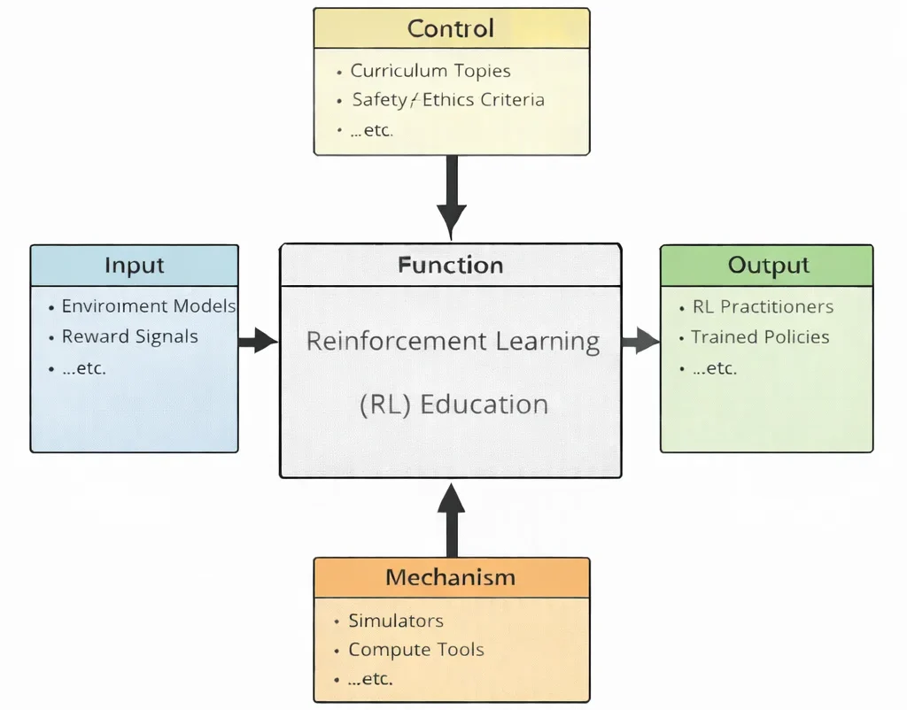
This IDEF0 (Input–Control–Output–Mechanism) diagram summarizes Reinforcement Learning (RL) Education as a structured learning system. Inputs on the left—environment models, reward signals, etc.—represent the foundations of RL, where learning is driven by interaction, feedback, and sequential decision-making. Controls at the top—curriculum topics, safety/ethics criteria, etc.—define what is taught and how competence is evaluated, while also imposing constraints that encourage responsible design and experimentation. The central function, Reinforcement Learning (RL) Education, transforms these inputs and controls into applied skill through guided study, experimentation, and iterative improvement of agents and policies. Outputs on the right—RL practitioners, trained policies, etc.—represent intended outcomes: learners who can design, train, and evaluate RL systems, and learned strategies that perform tasks effectively. Mechanisms at the bottom—simulators, compute tools, etc.—provide the enabling environment, including simulation platforms and computational resources used to run experiments safely and at scale.
Reinforcement Learning (RL) is a dynamic area within artificial intelligence and machine learning that models learning through interaction and feedback. Unlike approaches in data science and analytics, which extract patterns from static datasets, RL agents discover behaviours by acting in an environment and receiving rewards or penalties. This trial-and-error process enables strong performance in complex decision-making tasks such as game playing, autonomous navigation, and closed-loop control.
RL connects deeply with other AI areas: deep learning provides powerful function approximators; computer vision and natural language processing (NLP) give agents perception and language grounding. At scale, RL systems run on cloud computing with fit-for-purpose cloud deployment models.
In applied settings, RL is pivotal for robotics and autonomous systems, where agents must act safely under uncertainty. In smart manufacturing and Industry 4.0, it drives adaptive control and process optimisation; in IoT and smart technologies, RL closes feedback loops across networks of connected devices.
RL complements—and differs from—other paradigms. In supervised learning, models learn from labelled examples; in unsupervised learning, they discover structure in unlabelled data. RL instead builds policies from experiential feedback. It also augments expert systems by refining rule-based decisions with adaptive learning.
The relevance of RL is expanding alongside emerging technologies. It already supports space exploration technologies and satellite technology, and may ultimately benefit from advances in quantum computing, including qubits, superposition, and quantum gates.
Rooted in STEM and enriched by information technology, RL equips students to work at the frontier of intelligent decision-making—whether optimising supply chains, training self-driving vehicles, or supporting autonomy in critical systems.

Advanced Decision-Making Module
Explore our in-depth technical guides covering preference optimization, foundation model alignment, predictive world models, and multi-agent game theory:
- Reinforcement Learning from Human Feedback (RLHF) & AI Alignment
Master PPO surrogate loss, DPO log-ratio implicit reward, Bradley-Terry reward modeling, KL divergence penalties, and Constitutional AI. - Model-Based Reinforcement Learning & Sim-to-Real Transfer
Explore recurrent world models (Dreamer, RSSM), Model Predictive Control (MPC), domain randomization, and zero-shot robotic policy transfer. - Multi-Agent Reinforcement Learning (MARL) & Decentralized Coordination
Examine stochastic Markov games, Centralized Training with Decentralized Execution (CTDE), QMIX monotonic value factorization, and Nash Equilibrium.
Core Principles of Reinforcement Learning
Agents, Actions, and States
- Agent: The decision-making entity, such as a software program controlling a virtual character, or a physical robot navigating a room.
- States: The agent observes the state of the environment at each step. A state may include the agent’s position, objects it interacts with, or other relevant features.
- Actions: At any given state, the agent chooses an action from a set of possible actions. The outcome of that action changes the environment’s state and affects future decisions.
Rewards and Penalties
The environment provides feedback in the form of a numerical reward, which can be positive or negative. When the agent performs an action that advances its goals, it receives a positive reward; if it takes a counterproductive action, it might receive a penalty or a lower reward. Over time, the agent learns to associate certain actions in certain states with higher cumulative rewards.
Goal of Maximizing Cumulative Reward
The objective in reinforcement learning is not just to achieve an immediate reward but to maximize the sum of rewards over the long run. This focus on cumulative gain encourages the agent to develop strategies that balance short-term gains against long-term benefits. For instance, the agent might delay immediate gratification to secure more substantial rewards later.
Exploration vs. Exploitation
A key challenge in RL is the trade-off between exploration—trying new actions to discover potentially better rewards—and exploitation—using known strategies that have previously yielded good results. Finding an appropriate balance allows the agent to continually improve without getting stuck in suboptimal patterns of behavior.
Fundamental Techniques and Algorithms
This page covers the main families of RL methods. Use the quick map below to jump into the detailed sections you’ve added.
Value-Based Methods
Examples include Q-Learning, Double DQN, and Dueling DQN.
- Learn action-values, written as Q(s, a), and act greedily from the value estimates.
- Work well for discrete actions and tabular or pixel tasks with replay buffers.
Policy-Gradient Methods
Examples include REINFORCE and PPO.
- Directly optimise a stochastic policy, written as πθ(a | s), and handle continuous actions naturally.
- Use baselines and advantages to reduce variance; PPO adds clipping for stable updates.
See Policy Gradients & Actor–Critic
See Exploration & Intrinsic Motivation
Actor–Critic Methods
Examples include A2C, A3C, PPO, and SAC.
- The actor chooses actions, while the critic estimates value or advantage for lower-variance updates.
- SAC adds entropy regularisation and a learned temperature for smooth continuous control.
Model-Free vs. Model-Based
- Model-Free RL: learn policy or values directly from experience. It is usually simpler and robust, but more data-hungry.
- Model-Based RL: learn dynamics or reward models to plan or imagine data. It can be more sample-efficient, but needs careful model design and validation.
See Model-Based RL & World Models
Tip: If visitors only need a primer, keep this overview. For advanced readers, the deeper sections on exploration, shaping, curriculum, model-based learning, and diagnostics provide the full playbook.
Mathematical Foundations: MDPs & Bellman Equations
Markov Decision Processes (MDPs)
Reinforcement learning tasks are often modelled as a Markov Decision Process, or MDP. An MDP may be written as:
$$\mathcal{M} = \langle \mathcal{S}, \mathcal{A}, P, R, \gamma \rangle$$
Here, S is the set of possible states, A is the set of possible actions, P(s’ | s, a) describes the transition dynamics, R(s, a) represents the reward, and γ ∈ [0,1) is the discount factor. Some problems are episodic, meaning they end at a terminal state. Others are continuing, meaning the agent keeps acting without a clear final endpoint.
Returns, Policies, and Value Functions
- Return: the discounted future reward from a given time step:
$$G_t = \sum_{k=0}^{\infty} \gamma^{k} r_{t+k+1}$$
- Policy: the rule used by the agent to choose actions. A policy may be stochastic, written as π(a | s), or deterministic, written as μ(s).
- State value: the expected return starting from state s and following policy π:
$$V^{\pi}(s) = \mathbb{E}_{\pi}[G_t \mid S_t = s]$$
- Action value: the expected return after taking action a in state s, then following policy π:
$$Q^{\pi}(s,a) = \mathbb{E}_{\pi}[G_t \mid S_t = s, A_t = a]$$
- Advantage: how much better an action is compared with the average value of the state:
$$A^{\pi}(s,a) = Q^{\pi}(s,a) – V^{\pi}(s)$$
Bellman Equations
Bellman equations express the recursive structure of reinforcement learning. The value of a state depends on the immediate reward and the discounted value of the next state.
Bellman expectation equation for a fixed policy:
$$V^{\pi}(s) = \sum_{a} \pi(a \mid s) \left[ R(s,a) + \gamma \sum_{s’} P(s’ \mid s,a) V^{\pi}(s’) \right]$$
$$Q^{\pi}(s,a) = R(s,a) + \gamma \sum_{s’} P(s’ \mid s,a) \sum_{a’} \pi(a’ \mid s’) Q^{\pi}(s’,a’)$$
Bellman optimality equations:
$$V^{*}(s) = \max_{a} \left[ R(s,a) + \gamma \sum_{s’} P(s’ \mid s,a) V^{*}(s’) \right]$$
$$Q^{*}(s,a) = R(s,a) + \gamma \sum_{s’} P(s’ \mid s,a) \max_{a’} Q^{*}(s’,a’)$$
Dynamic Programming: When the Model Is Known
- Policy evaluation: repeatedly apply the Bellman expectation equation to estimate Vπ for a fixed policy.
- Policy improvement: update the policy by choosing actions that look best according to the current value estimates, such as:
$$\pi_{\text{new}}(s) = \arg\max_a Q^{\pi}(s,a)$$
- Policy iteration: alternate between policy evaluation and policy improvement until the policy becomes stable.
- Value iteration: repeatedly apply the Bellman optimality equation until the value function approaches V*.
Temporal-Difference Learning: Learning from Samples
Temporal-difference learning estimates values from experience, without needing a complete model of the environment. It combines immediate reward with a bootstrapped estimate of future value.
TD(0) state-value update:
$$V(S_t) \leftarrow V(S_t) + \alpha \left[ r_{t+1} + \gamma V(S_{t+1}) – V(S_t) \right]$$
Q-learning: off-policy control
$$Q(S_t,A_t) \leftarrow Q(S_t,A_t) + \alpha \left[ r_{t+1} + \gamma \max_{a’} Q(S_{t+1},a’) – Q(S_t,A_t) \right]$$
SARSA: on-policy control
$$Q(S_t,A_t) \leftarrow Q(S_t,A_t) + \alpha \left[ r_{t+1} + \gamma Q(S_{t+1},A_{t+1}) – Q(S_t,A_t) \right]$$
Practical notes
- The effective planning horizon is approximately 1 / (1 – γ), so choose γ to match the timescale of the task.
- Reward shaping should be used cautiously. Potential-based shaping can preserve the optimal policy when the added shaping term has the form:
$$F(s,s’) = \gamma \Phi(s’) – \Phi(s)$$
- Normalise returns where appropriate, and watch for bootstrapping instability caused by an unsuitable learning rate α.
- Keep exploration behaviour, such as ε-greedy action selection, separate from final evaluation, where the policy may be tested greedily.
Policy Gradients & Actor–Critic with PPO and GAE
Value-based methods, such as Q-learning, search for a good policy indirectly by first learning value estimates and then acting greedily. Policy-gradient methods go straight for the goal: they adjust a parameterised policy πθ(a | s) to maximise expected return.
This is especially useful for large action spaces, continuous control, and policies that must remain stochastic in order to keep exploring or represent mixed behaviours.
Objective and the Log-Trick
The performance objective can be written as:
$$J(\theta) = \mathbb{E}_{\tau \sim \pi_{\theta}} \left[ \sum_{t=0}^{T-1} \gamma^t r_{t+1} \right]$$
Here, a trajectory τ is sampled by running the policy πθ. Using the log-derivative identity, the policy-gradient theorem gives:
$$\nabla_{\theta} J(\theta) = \mathbb{E}_{\pi_{\theta}} \left[ \sum_{t=0}^{T-1} \nabla_{\theta} \log \pi_{\theta}(A_t \mid S_t) G_t \right]$$
The intuition is simple: increase the probability of actions that led to higher return, and decrease the probability of actions that performed poorly.
Variance Reduction: Baselines and Advantages
Directly using Gt can be unbiased but noisy. A baseline b(St) can be subtracted without changing the expected gradient:
$$\nabla_{\theta} J(\theta) = \mathbb{E}_{\pi_{\theta}} \left[ \sum_t \nabla_{\theta} \log \pi_{\theta}(A_t \mid S_t) \left( G_t – b(S_t) \right) \right]$$
A practical baseline is the value function Vπ(St), producing the advantage:
$$A^{\pi}(S_t,A_t) = G_t – V^{\pi}(S_t)$$
The advantage asks: “How much better was this action than expected from this state?”
REINFORCE: Monte Carlo Policy Gradient
- Collect full episodes using the current policy πθ.
- Compute returns Gt, or advantages Gt – b(St).
- Update the policy parameters:
$$\theta \leftarrow \theta + \alpha \sum_t \nabla_{\theta} \log \pi_{\theta}(A_t \mid S_t) \left( G_t – b(S_t) \right)$$
Strength: REINFORCE is simple and unbiased.
Limitation: it often has high variance and can learn slowly. This is why practical agents often add a critic to supply a stronger baseline and use bootstrapping.
Actor–Critic: Learning a Policy and a Value Function Together
Actor–critic methods use two learned components. The actor is the policy πθ, which chooses actions. The critic is the value function Vw, which estimates how good a state is.
At each step, the method forms a temporal-difference error:
$$\delta_t = r_{t+1} + \gamma V_w(S_{t+1}) – V_w(S_t)$$
This TD error is a low-variance estimate of the advantage.
- Critic update: train the critic by regression toward a TD target:
$$w \leftarrow w – \alpha_v \nabla_w \left( V_w(S_t) – \left[ r_{t+1} + \gamma V_w(S_{t+1}) \right] \right)^2$$
- Actor update: update the policy using the estimated advantage:
$$\theta \leftarrow \theta + \alpha_{\pi} \nabla_{\theta} \log \pi_{\theta}(A_t \mid S_t) \hat{A}_t$$
where Ât may be δt or a multi-step advantage estimate.
Generalized Advantage Estimation (GAE)
Generalized Advantage Estimation, or GAE, trades bias for variance using a smoothing parameter λ ∈ [0,1]. First define the TD residual:
$$\delta_t = r_{t+1} + \gamma V_w(S_{t+1}) – V_w(S_t)$$
Then accumulate advantage estimates as:
$$\hat{A}_t = \sum_{l=0}^{\infty} (\gamma \lambda)^l \delta_{t+l}$$
Rule of thumb: λ ≈ 0.95 often works well. A lower λ can reduce variance but may increase bias.
PPO: Stable Actor–Critic Updates
Proximal Policy Optimisation, or PPO, limits how much each update can change the policy. This makes actor–critic training more stable.
Let the probability ratio be:
$$r_t(\theta) = \frac{\pi_{\theta}(A_t \mid S_t)}{\pi_{\theta_{\text{old}}}(A_t \mid S_t)}$$
The clipped surrogate objective is:
$$L^{\text{clip}}(\theta) = \mathbb{E} \left[ \min(r_t(\theta)\hat{A}_t, \mathrm{clip}(r_t(\theta), 1-\epsilon, 1+\epsilon)\hat{A}_t) \right]$$
The total PPO loss often combines actor loss, critic loss, and an entropy bonus:
$$\mathcal{L}(\theta,w) = – L^{\text{clip}}(\theta) + c_v \mathbb{E} \left[ \left( V_w(S_t) – \hat{V}_t \right)^2 \right] – c_e \mathbb{E} \left[ \mathcal{H} \left( \pi_{\theta}(\cdot \mid S_t) \right) \right]$$
Here, V̂t = Vw(St) + Ât or a multi-step return. The entropy term H encourages exploration. A common range for the clipping parameter is ε ∈ [0.1, 0.3].
Putting PPO together in plain English
- Run the current policy for N steps across M environments. Store St, At, rt+1, St+1, and log πθold(At | St).
- Compute value estimates Vw(St) and advantages Ât, often using GAE. Normalise Ât to zero mean and unit standard deviation.
- For several epochs, shuffle the collected data and update the actor, critic, and entropy terms.
- Set θold ← θ, then repeat the process.
When to Use Each Method
- REINFORCE: conceptually simple and useful for small problems or as a teaching baseline.
- Actor–Critic methods: faster than plain Monte Carlo policy gradients because they use TD-based advantage estimates.
- PPO with GAE: robust and widely used for continuous control tasks such as robotics and locomotion, as well as many discrete-action tasks.
Practical Tips That Save Days of Debugging
- Normalise advantages per update batch to stabilise the actor step.
- Clip policy updates in PPO, and clip value targets if needed to avoid exploding losses.
- Use an entropy schedule: start higher to encourage exploration, then decay as learning progresses.
- For continuous actions: model πθ as a factorised Gaussian. Learn the mean and log standard deviation. If actions are bounded, squash with tanh and correct the log probability.
- Scale or normalise rewards where appropriate. Potential-based reward shaping may help:
$$F(s,s’) = \gamma \Phi(s’) – \Phi(s)$$
- Track diagnostics: explained variance of the critic, KL divergence, clip fraction, advantage statistics, value loss, and episode returns. If KL spikes or the clip fraction is near 0 or 1, tune the learning rate or ε.
Exploration Strategies & Intrinsic Motivation
Reinforcement learning agents must discover high-reward behaviours. Good exploration balances trying new actions with exploiting what already works. This section moves from classic bandit ideas to entropy-regularised learning and curiosity-driven methods, with plain-English guidance and the key equations.
1. Bandit and Tabular Foundations
- ε-greedy exploration: with probability ε, choose a random action; otherwise choose the action with the highest estimated value:
$$a = \arg\max_a Q(s,a)$$
A common approach is to reduce ε gradually, such as from 0.2–0.5 down to 0.01–0.05.
- Boltzmann or softmax exploration: actions are selected with probabilities based on their estimated values:
$$\pi(a \mid s) = \frac{\exp(Q(s,a)/\tau)}{\sum_{a’} \exp(Q(s,a’)/\tau)}$$
Here, τ is the temperature. A high temperature encourages wider exploration; a lower temperature makes the policy more greedy.
- Upper Confidence Bound (UCB): in bandit problems, UCB adds an optimism bonus to less-tested actions:
$$a_t = \arg\max_a \left[ \hat{Q}(a) + c \sqrt{\frac{\ln t}{n(a)}} \right]$$
The bonus shrinks as the number of trials n(a) grows.
- Optimistic initial values: set the initial value Q0 high so that unfamiliar actions look promising. This forces the agent to try different actions early instead of settling too quickly.
2. Entropy-Regularised Reinforcement Learning
Entropy-regularised reinforcement learning adds an entropy term to encourage stochastic policies and avoid premature collapse into narrow behaviour. For state St, policy π, and temperature α > 0, the objective can be written as:
$$J_{\alpha}(\pi) = \mathbb{E} \left[ \sum_{t=0}^{T-1} \gamma^t \left( r_{t+1} + \alpha \mathcal{H}(\pi(\cdot \mid S_t)) \right) \right]$$
where the entropy of the policy is:
$$\mathcal{H}(\pi(\cdot \mid s)) = – \sum_a \pi(a \mid s) \log \pi(a \mid s)$$
- PPO entropy bonus: PPO can include an entropy bonus in the loss to keep the policy exploratory, especially early in training.
- Soft Actor–Critic (SAC): SAC formalises entropy-regularised learning through soft value estimates:
$$V(s) = \mathbb{E}_{a \sim \pi} \left[ Q(s,a) – \alpha \log \pi(a \mid s) \right]$$
- Temperature learning: SAC can learn the temperature α by adjusting it toward a target entropy:
$$\mathcal{L}(\alpha) = \mathbb{E}_{a \sim \pi} \left[ -\alpha \left( \log \pi(a \mid s) + \mathcal{H}_{\text{target}} \right) \right]$$
A typical target entropy for continuous control is approximately the negative of the action dimension.
3. Intrinsic Motivation: Novelty and Curiosity Bonuses
For sparse or deceptive tasks, an agent may need an internal reason to explore. Intrinsic motivation adds an internal reward for novelty, surprise, or learning progress. The total reward may be written as:
$$r_t^{\text{total}} = r_t^{\text{ext}} + \beta r_t^{\text{int}}$$
Here, rtext is the external task reward, rtint is the intrinsic reward, and β controls how strongly curiosity influences learning. The scale of β is important: if it is too small, curiosity has little effect; if it is too large, the agent may chase novelty instead of solving the real task.
3.1 Count-Based Exploration
In tabular settings, a simple novelty bonus can be based on how often a state has been visited:
$$r^{\text{int}}(s) = \frac{\beta}{\sqrt{N(s)}}$$
where N(s) is the visit count for state s. Less-visited states receive a larger intrinsic reward.
For large observation spaces, pseudo-counts can be estimated using a density model. If ρt(x) is the model probability before seeing x, and ρ’t(x) is the probability after a one-step update on x, then a pseudo-count may be written as:
$$\hat{N}(x) = \frac{\rho_t(x)\left(1-\rho’_t(x)\right)}{\rho’_t(x)-\rho_t(x)}$$
The intrinsic reward can then be written as:
$$r^{\text{int}}(x) = \frac{\beta}{\sqrt{\hat{N}(x)+\epsilon}}$$
3.2 Curiosity Through Intrinsic Curiosity Module (ICM)
The Intrinsic Curiosity Module maps states into feature vectors φ(s). It then uses two models:
- Inverse model: predicts the action at from the feature pair (φ(st), φ(st+1)). This encourages features that are connected to controllable changes.
- Forward model: predicts the next feature vector from the current feature vector and action.
The intrinsic reward is based on the forward prediction error:
$$r_t^{\text{int}} = \eta \left\| \phi(s_{t+1}) – f(\phi(s_t),a_t) \right\|_2^2$$
A larger prediction error means the next state was more surprising in feature space. In practice, the bonus should be normalised and scaled carefully.
3.3 Random Network Distillation (RND)
Random Network Distillation keeps a fixed, randomly initialised target network ft(s). A predictor network fp(s) is trained to match it. Novel states are harder to predict, so they produce a larger error:
$$r_t^{\text{int}} = \eta \left\| f_{\text{p}}(s_t) – f_{\text{t}}(s_t) \right\|_2^2$$
RND can work well in hard-exploration tasks, but the intrinsic reward should be normalised. If the predictor overfits too quickly, the novelty bonus may vanish before the agent has learned useful behaviour.
Implementation Notes and Pitfalls
- Log rewards separately: track extrinsic reward, intrinsic reward, and total reward. Evaluate the final policy with intrinsic reward turned off.
- Normalise intrinsic bonuses: use running mean and standard deviation where appropriate, and clip unusually large bonuses.
- Schedule β: start with stronger exploration pressure, then reduce it as external rewards become more informative.
- Continuous control: keep the Gaussian policy standard deviation above a sensible floor. In PPO, do not anneal entropy too quickly.
- Noisy networks and parameter noise: injecting noise into weights can create more coherent exploration across states than adding random noise directly to each action.
- Bootstrapped heads: in DQN-style methods, multiple heads can approximate Thompson sampling and encourage varied exploration.
- Watch for reward hacking: curiosity can dominate learning if the agent finds a way to stay “surprised” without making real progress.
4. Safe Exploration with Constraints
In safety-sensitive settings, exploration must be constrained. If there is a per-step cost ct, such as collision, rule violation, or excessive force, the policy may be required to keep the long-run cost below a limit d:
$$J_C(\pi) \le d$$
A Lagrangian form can penalise policies that exceed the constraint:
$$\max_{\pi} \; J(\pi) – \lambda \left( J_C(\pi)-d \right)$$
The multiplier λ ≥ 0 can be updated online:
$$\lambda \leftarrow \left[ \lambda + \eta_{\lambda} \left( J_C(\pi)-d \right) \right]_+$$
In practice, the reward can be shaped as:
$$r_t^{\text{safe}} = r_t^{\text{ext}} – \lambda c_t$$
This encourages the agent to improve task performance while respecting safety-related costs.
5. Practical Recipes
- PPO with entropy bonus: a useful starting point for both discrete and continuous tasks. Typical clip values may be around ε = 0.1 to 0.2, with entropy coefficient ce = 0.01 to 0.05.
- SAC for continuous control: a strong default when stable exploration and continuous actions matter. A common target entropy is approximately -action dimension.
- Curiosity methods: start with RND for hard-exploration games or ICM for control tasks with meaningful state transitions. Set β so intrinsic returns are roughly 10% to 50% of extrinsic returns early in training.
- Count bonuses: for grid worlds or discrete observations, rint = β / sqrt(N(s)) is often a strong baseline.
- Diagnostics: plot state-visit heatmaps, pseudo-counts, KL divergence to the old policy, advantage statistics, and the ratio of intrinsic reward to total reward over time.
Reward Shaping, Curriculum Learning & Domain Randomization
The goal of this stage is to make reinforcement learning more efficient, more stable, and more transferable. A good RL system should not only learn faster; it should also learn the right behaviour, generalise beyond a narrow training setup, and avoid unsafe shortcuts.
1. Reward Shaping: Helping the Agent Without Changing the Goal
Reward shaping adds extra guidance to the reward signal so that the agent receives useful feedback before it reaches the final goal. This can speed up learning, especially when the true reward is sparse or delayed.
A safe form is potential-based shaping, which adds a term based on a potential function Φ(s):
$$r'(s,a,s’) = r(s,a,s’) + \gamma \Phi(s’) – \Phi(s)$$
The intuition is that the agent receives extra reward when it moves toward more promising states, but the true optimal policy is preserved if the shaping is designed carefully.
- Useful choices for Φ(s): negative distance to the goal, estimated value of a state, or progress toward a clearly defined target.
- Risky choices: rewards for behaviours that can be exploited, such as spinning, shaking, repeating easy actions, or triggering sensors without solving the real task.
- Practical advice: use shaping to guide early learning, then reduce its influence so the final policy is judged mainly by the true task reward.
2. Curriculum Learning: Making Hard Tasks Learnable
Curriculum learning presents tasks in a planned sequence, starting with easier versions and gradually increasing difficulty. This mirrors how humans learn complex skills: first simplify the problem, then remove the scaffolding.
- Start near success: begin with easier starting positions, shorter distances, fewer obstacles, or simpler goals.
- Increase difficulty gradually: widen the starting region, add more environmental variation, or lengthen the required planning horizon.
- Use success rate as feedback: if the agent succeeds too easily, increase difficulty; if it fails too often, reduce difficulty.
A simple adaptive curriculum can aim to keep the success rate in a useful training range, such as 60% to 80%, where the task is challenging but not impossible.
3. Domain Randomization: Preparing for Real-World Variation
Domain randomization exposes the agent to many versions of the environment during training. Instead of training on one fixed simulation, the system randomizes physical, visual, or sensor-related properties so the learned policy becomes more robust.
- Physical parameters: mass, friction, gravity, delays, joint limits, actuator strength, and object size.
- Sensor parameters: noise, bias, missing readings, camera angle, lighting, and calibration error.
- Initial conditions: starting position, goal location, obstacle placement, and environmental layout.
This is especially important for sim-to-real transfer. A policy trained only in a perfect simulator may fail when the real world is slightly different. A policy trained across many variations is more likely to tolerate uncertainty.
4. Practical Playbook
- Early training: use sparse reward plus light potential shaping, easy curriculum settings, and moderate randomization.
- Middle training: reduce shaping, increase task difficulty, and widen randomization ranges.
- Late training: evaluate mostly on the true reward, realistic task settings, and held-out randomization conditions.
Good plots to monitor include success versus difficulty, training return versus held-out return, and the proportion of shaped reward compared with true reward over time.
Exploration Cookbook: Defaults and Pitfalls
Exploration methods should be chosen according to the task type. Simple discrete problems may only need ε-greedy exploration, while continuous control problems often benefit from entropy-regularised methods such as SAC or PPO with an entropy bonus.
| Method | Useful When | Key Idea | Watch-Out |
|---|---|---|---|
| ε-greedy | Discrete actions and simple baselines | Take a random action with probability ε, otherwise act greedily. | Reducing ε too quickly can cause premature exploitation. |
| Softmax / Boltzmann | Discrete actions where smoother exploration is useful | Sample actions according to a probability distribution based on Q-values. | A high temperature may cause dithering; a low temperature may collapse too soon. |
| Entropy bonus | Policy-gradient methods such as PPO | Reward the policy for remaining sufficiently stochastic. | Too much entropy can make behaviour noisy and unfocused. |
| SAC temperature | Continuous control tasks | Balance reward maximisation with policy entropy. | Temperature and action standard deviation should be monitored carefully. |
| Count bonus | Small state spaces or grid worlds | Reward less-visited states more strongly. | Does not scale well to very large observation spaces. |
| RND or ICM curiosity | Sparse-reward or hard-exploration tasks | Give intrinsic reward for novelty or prediction error. | The agent may chase novelty instead of solving the real task. |
| Safe exploration | Robotics, vehicles, or safety-critical control | Use costs, penalties, or constraints to limit unsafe behaviour. | Evaluate true constraint satisfaction, not just reward. |
Quick recipe: start with PPO plus entropy bonus for many general tasks. For continuous control, try SAC. In sparse-reward tasks, add curiosity carefully and evaluate with intrinsic reward turned off.
Model-Based Reinforcement Learning and World Models
Model-based reinforcement learning learns a model of the environment and then uses that model to plan, imagine extra experience, or improve sample efficiency. Instead of learning only from real interaction, the agent can ask, “What might happen if I take this action?”
1. Learning the Dynamics and Reward Model
A model can learn to predict the next state and reward from the current state and action:
$$\hat{s}_{t+1} = f_{\theta}(s_t,a_t)$$
$$\hat{r}_t = r_{\xi}(s_t,a_t,\hat{s}_{t+1})$$
- One-step accuracy checks whether the model predicts the next state correctly.
- Multi-step accuracy checks whether the model remains reliable over longer imagined rollouts.
- Ensembles can estimate uncertainty by comparing predictions from several models.
2. Planning with MPC and CEM
Model Predictive Control, or MPC, plans over a short horizon, executes only the first action, then replans at the next step. This reduces the danger of relying too heavily on long, imperfect model predictions.
The Cross-Entropy Method, or CEM, searches for good action sequences by sampling many candidate sequences, keeping the best ones, and updating the sampling distribution toward those elites.
# Inputs: learned model, reward model, value estimate

# Choose horizon H, population N, elite size M, and iterations L


for each real environment step:

    sample N candidate action sequences

    simulate each sequence using the learned model

    score each sequence using predicted reward and value tail

    keep the top M elite sequences

    refit the sampling distribution toward the elites

    execute only the first action

    observe the real next state

    replan from the new state
In real systems, short horizons such as H = 5 to 20 are often safer than long imagined rollouts, especially when the learned model is imperfect.
3. MBPO and Dyna-Style Short Rollouts
Dyna-style methods use a learned model to generate imagined data, then train the policy or value function using both real and imagined experience. MBPO-style approaches keep imagined rollouts short, often only 1 to 5 steps, to reduce model-bias accumulation.
- Use short rollouts: long imagined rollouts may drift away from realistic states.
- Refresh imagined data often: as the real replay buffer grows, update the model and regenerate imagined samples.
- Compare real and imagined returns: if imagined data looks good but real performance does not improve, the model may be misleading the learner.
4. Dreamer-Style World Models
World-model approaches learn a compact latent representation of the environment. Instead of planning directly in raw pixels or high-dimensional observations, the agent learns an internal state space and trains the actor and critic through imagined trajectories inside that space.
- Encoder: maps observations into latent states.
- Latent dynamics model: predicts how latent states change after actions.
- Reward model: predicts reward from latent states and actions.
- Actor and critic: learn from imagined trajectories generated by the world model.
This is useful for pixel-based control and partially observable tasks, but it requires careful tuning and diagnostics to avoid model collapse or misleading imagined experience.
5. Handling Model Uncertainty
A learned model is never perfect. Model uncertainty can be estimated using ensembles, and plans that pass through uncertain regions can be penalized:
$$\tilde{r} = \hat{r} – \beta |\sigma_{\text{model}}|$$
This discourages the agent from exploiting areas where the model is unsure. It is especially important in offline RL and sim-to-real transfer.
Choosing a Model-Based Method
| Method | Best For | Strength | Watch-Out |
|---|---|---|---|
| MPC + CEM | Real-time control and short-horizon planning | Replans frequently and can include safety constraints directly. | Needs fast model inference and can suffer from model bias at long horizons. |
| MBPO / Dyna | Continuous-control tasks with moderate observations | Uses short imagined rollouts to improve sample efficiency. | Too much imagined data can train the agent on model errors. |
| Dreamer-style world models | Pixel-based control and partially observable tasks | Learns and trains in a compact latent imagination space. | More complex implementation and requires careful latent-model diagnostics. |
Tuning Checklist: Quick Wins and Fixes
MPC + CEM
- Start with: horizon H = 10 to 15, population N = 512, elite size about 10% to 20%, and 3 to 5 inner iterations.
- If real return is poor: shorten the planning horizon, add a value tail, or penalize model uncertainty.
- If plans are too similar: increase population size or initial search variance.
- If control is jittery: smooth actions, penalize acceleration, or use lower-dimensional control points.
MBPO / Dyna
- Start with: imagined rollout length K = 1 to 5.
- If learning stalls: shorten imagined rollouts and rely more on real data.
- If the critic becomes unstable: reduce imagined data ratio or retrain the model more often.
- If validation model error grows: collect more real data or use an ensemble.
Dreamer-Style World Models
- Start with: short imagination horizons and stable latent representations.
- If the model reconstructs poorly: adjust the encoder, decoder, or latent capacity.
- If the actor exploits imagination errors: shorten the imagination horizon or strengthen regularization.
- If training becomes unstable: check reward scale, value loss, KL terms, and latent-state statistics.
Diagnostics and Debugging
Reinforcement learning can fail silently. A policy may appear to learn, but the improvement may come from reward hacking, lucky random seeds, unstable value estimates, or an unrealistic simulator. Diagnostics help distinguish genuine learning from accidental progress.
- Episode return: track mean, median, and spread across seeds.
- Policy entropy: check whether the policy is exploring too much or collapsing too early.
- KL divergence and clipping fraction: useful for PPO stability.
- Value loss and explained variance: show whether the critic is learning useful value estimates.
- Advantage statistics: unstable advantage values often indicate reward scaling or value-estimation problems.
- Intrinsic versus extrinsic reward: check whether curiosity is helping or dominating.
- State coverage: heatmaps or visit counts reveal whether the agent explores the important parts of the environment.
- Real versus imagined performance: for model-based methods, compare planned values with realized returns.
Practical Applications and Examples
Game Playing
Reinforcement learning became widely known through game-playing systems. Agents can learn strategies by repeatedly playing games, receiving rewards for success, and improving through trial and error. This has been demonstrated in board games, video games, and simulated strategic environments.
Robotics and Autonomous Navigation
In robotics, RL can help robots learn control policies for manipulation, locomotion, and navigation. A robot may learn to grasp an object, avoid obstacles, or adapt to changing surroundings through repeated interaction with a simulator or carefully controlled real-world environment.
Benefits and Challenges
Benefits
- Adaptability: RL agents can improve as they gain experience.
- Flexibility: RL applies to tasks where fixed rules or labelled examples are difficult to provide.
- Sequential decision-making: RL is well suited to problems where current actions affect future outcomes.
- Closed-loop control: RL can support systems that must act, observe, and adjust repeatedly.
Challenges
- Data efficiency: RL may require many interactions, which can be expensive or unsafe in the real world.
- Stability: training can be sensitive to hyperparameters, reward design, and exploration strategy.
- Safety: unsafe exploration is unacceptable in areas such as autonomous driving, healthcare, and industrial control.
- Reward design: poorly designed rewards can produce unwanted or misleading behaviour.
- Generalization: a policy that works in one environment may fail when conditions change.
Advancing the Field
Researchers are working to make reinforcement learning more sample-efficient, interpretable, reliable, and aligned with human values. Important directions include hierarchical reinforcement learning, transfer learning, offline reinforcement learning, safe reinforcement learning, and better evaluation methods.
These advances aim to move RL beyond benchmark tasks and into systems that can learn responsibly in complex real-world environments.
Reinforcement Learning: Conclusion
Reinforcement Learning is a powerful framework for decision-making and control. Agents learn by interacting with an environment, receiving feedback, and gradually improving their behaviour. Beyond benchmark games, modern RL supports safe autonomy in robotics, adaptive control in industry, and closed-loop optimisation across networked systems.
- It is more than an algorithm: success depends on reward design, exploration, data pipelines, diagnostics, and robust evaluation.
- Choosing the right tool matters: PPO and SAC are strong baselines, while model-based methods such as MPC, MBPO, and Dreamer trade extra complexity for sample efficiency.
- Safe learning is essential: curricula, constraints, domain randomization, and careful reward shaping help reduce reckless behaviour.
- Measurement matters: track returns, entropy, KL divergence, value loss, model error, and reproducibility across seeds.
As compute, simulators, sensors, and modelling tools improve, reinforcement learning will continue to shape intelligent systems that can learn, adapt, and act in complex changing environments.
Next steps: review Diagnostics and Debugging, revisit the Exploration Cookbook, or connect this topic with Robotics and Autonomous Systems and the broader AI and Machine Learning hub.
Why Study Reinforcement Learning
Understanding How Machines Learn Through Interaction
Reinforcement Learning (RL) is a branch of artificial intelligence that focuses on how agents learn to make decisions by interacting with their environment and receiving feedback in the form of rewards or penalties. For students preparing for university, studying RL offers an exciting opportunity to explore how intelligent behavior can emerge from trial and error, and how machines can learn optimal strategies in dynamic and uncertain settings.
Exploring Core Concepts in Decision-Making and Control
RL introduces students to essential ideas such as agents, environments, states, actions, rewards, policies, and value functions. They learn how algorithms like Q-learning, SARSA, and policy-gradient methods help agents improve their performance over time. These concepts are foundational not only for AI, but also for understanding systems that involve learning, adaptation, and decision-making under uncertainty.
Building Intelligent Systems for Real-World Applications
Reinforcement learning powers many real-world innovations, including autonomous vehicles, game-playing AI systems, robotic control systems, personalised recommendations, and resource optimisation tools. Students gain practical insight into how RL can be used to develop adaptive systems that improve their performance through experience, without needing explicit instruction for every situation.
Connecting Theory with Experimentation and Simulation
RL combines mathematical modelling with hands-on experimentation in simulated environments. Students explore the balance between exploration and exploitation, tune learning rates, and evaluate agent performance in different scenarios. Simulation tools and reinforcement learning libraries allow learners to test and visualise learning behaviour in controlled settings, reinforcing theoretical knowledge with interactive experience.
Preparing for Advanced Study and Emerging Careers in AI
A background in reinforcement learning supports further academic study in artificial intelligence, robotics, neuroscience, operations research, and behavioural economics. It also opens pathways to careers in AI development, automation, financial modelling, simulation, game design, and intelligent control systems. For university-bound students, studying reinforcement learning offers a window into how machines can learn autonomously—an area of research and innovation with profound future potential.
Key Terms in Reinforcement Learning
The following terms help students understand the basic language of reinforcement learning. Each concept describes part of the learning loop between an agent and its environment.
- Agent
- The learner or decision-maker. It may be a software agent, robot, game-playing system, control algorithm, or simulated learner.
- Environment
- The world in which the agent acts. The environment responds to the agent’s actions and provides new states and rewards.
- State
- The information available to the agent at a particular moment. A state may include position, sensor readings, game board layout, system condition, or other relevant features.
- Action
- A choice made by the agent. Actions may be discrete, such as moving left or right, or continuous, such as applying a steering angle or motor force.
- Reward
- The feedback signal that tells the agent whether an action was useful. Rewards guide learning, but they must be designed carefully to avoid unintended behaviour.
- Policy
- The rule or strategy the agent uses to choose actions. A policy may be deterministic or probabilistic.
- Value Function
- An estimate of how good a state is, based on the expected future reward from that state.
- Q-Value
- An estimate of how good it is to take a particular action in a particular state, considering both immediate and future rewards.
- Exploration
- The process of trying new actions to discover better strategies or learn more about the environment.
- Exploitation
- The process of using actions already known to produce good results.
- Episode
- One complete run of a task, from the starting condition to a terminal condition or stopping point.
- Return
- The total future reward received over time, often discounted so that nearer rewards count more strongly than distant rewards.
Reinforcement Learning: Review Questions and Answers
1. What is Reinforcement Learning?
Answer: Reinforcement learning is a branch of machine learning in which an agent learns to make decisions by interacting with an environment. It receives feedback in the form of rewards or penalties that guide its behaviour over time. This trial-and-error approach helps the agent improve its performance based on accumulated experience. RL is widely used for tasks involving sequential decision-making and dynamic environments.
2. How does reinforcement learning differ from supervised learning?
Answer: In supervised learning, a model learns from labelled examples that show the correct answer. In reinforcement learning, the agent does not usually receive a correct answer for every action. Instead, it acts in an environment and receives rewards or penalties. The agent must discover which actions lead to better long-term outcomes through interaction and feedback.
3. What are the key components of a reinforcement learning system?
Answer: A reinforcement learning system typically includes an agent, an environment, states, actions, and a reward function. The agent follows a policy that maps states to actions, while the environment provides feedback through rewards and state transitions. Value functions and models of state transitions may also help estimate long-term benefits. Together, these components allow the agent to learn and refine its behaviour through repeated updates.
4. What is the role of reward functions in reinforcement learning?
Answer: The reward function provides the main feedback signal in reinforcement learning. It quantifies the immediate benefit or cost of an action, guiding the agent toward behaviours that maximise cumulative reward. A well-designed reward function is critical because it aligns the agent’s behaviour with the actual goal of the task. A poorly designed reward can lead to unintended or misleading behaviour.
5. What is the difference between value-based and policy-based methods in reinforcement learning?
Answer: Value-based methods estimate the value of states or state-action pairs and then derive a policy from those value estimates. Q-learning is a common example. Policy-based methods directly optimise the policy itself, adjusting how actions are selected based on performance. Each approach has strengths depending on the type of task, action space, and stability requirements.
6. How do exploration and exploitation trade-offs affect reinforcement learning?
Answer: The exploration-exploitation trade-off is central to reinforcement learning. Exploration means trying new actions to discover potentially better strategies, while exploitation means using actions already known to give good results. Too much exploration can slow learning, but too much exploitation can trap the agent in a suboptimal strategy. A good RL system must balance both.
7. What is Q-learning?
Answer: Q-learning is a value-based reinforcement learning algorithm that estimates the best action-value function for state-action pairs. It updates Q-values using a Bellman-style equation that combines immediate reward with estimated future reward. Because it is off-policy, it can learn an optimal policy even while following an exploratory behaviour policy during training.
8. How can reinforcement learning be applied in real-world scenarios?
Answer: Reinforcement learning can be applied in robotics, autonomous vehicles, finance, game playing, industrial control, recommendation systems, and resource optimisation. It is useful when decisions must be made sequentially and when current actions affect future outcomes. For example, a robot may learn how to navigate complex terrain, while an industrial control system may learn how to optimise energy use over time.
9. What are some challenges associated with reinforcement learning algorithms?
Answer: RL algorithms often face high sample complexity, meaning they may need many interactions before learning effective behaviour. They may also struggle with stability and convergence, especially when rewards are sparse, delayed, or noisy. Managing exploration and exploitation can be difficult, and scaling RL to high-dimensional or continuous action spaces remains an active research challenge.
10. How does reinforcement learning contribute to advancements in AI and decision-making?
Answer: Reinforcement learning contributes to AI by providing a framework in which systems can learn effective behaviour through direct interaction with their environments. It has supported breakthroughs in strategic games, robotics, adaptive control, and optimisation. RL also enables autonomous systems to adapt to changing conditions and make decisions without requiring explicit instructions for every possible situation.
Reinforced Learning: Thought-Provoking Questions and Answers
1. How can reinforcement learning be integrated with other AI paradigms to solve complex real-world problems?
Answer: Reinforcement learning can be combined with deep learning to form deep reinforcement learning, allowing agents to process high-dimensional inputs such as images, sensor data, or complex system states. Deep learning helps extract useful features from raw data, while reinforcement learning helps the agent choose actions through feedback and experience.
Reinforcement learning can also be integrated with supervised and unsupervised learning. Supervised learning may provide labelled examples that guide early training, while unsupervised learning can discover useful patterns or state representations before the agent begins decision-making. This hybrid approach can reduce training time, improve generalisation, and make AI systems more resilient in complex environments.
2. In what ways could advancements in reinforcement learning revolutionize personalized learning experiences?
Answer: Reinforcement learning could support adaptive educational platforms that adjust content, difficulty, timing, and feedback according to each learner’s progress. Instead of giving all students the same pathway, an RL-based system could observe how a student responds and then recommend the next most useful exercise, explanation, or challenge.
Such systems could also improve intelligent tutoring by testing different teaching strategies over time. If a learner struggles with a topic, the system may switch to simpler examples, visual explanations, or spaced revision. If the learner is progressing quickly, it may increase difficulty. This could make digital learning more responsive, personal, and engaging.
3. What ethical considerations emerge from deploying reinforcement learning in autonomous decision-making systems?
Answer: Reinforcement learning in autonomous systems raises serious ethical questions about accountability, transparency, fairness, and safety. If an RL system makes decisions that affect people’s lives, users and regulators need to know how those decisions are made, what data shaped the system, and who is responsible when outcomes go wrong.
There is also a risk that an agent may optimise the wrong objective. If rewards are poorly designed, the system may find shortcuts that appear successful in technical terms but cause unfair, unsafe, or harmful consequences. This is why reinforcement learning requires clear ethical guidelines, careful testing, human oversight, and regulatory frameworks when used in high-impact settings.
4. How might the scalability challenges of reinforcement learning be addressed in large-scale, dynamic environments?
Answer: Scalability challenges can be addressed using methods such as hierarchical learning, distributed training, transfer learning, and more efficient actor–critic algorithms. Hierarchical learning breaks a complex task into smaller sub-tasks, making the problem easier to learn. Distributed training allows many simulations or agents to collect experience in parallel, speeding up learning.
Transfer learning can also reduce the need to learn from scratch. If an agent has already learned useful behaviour in one environment, that knowledge may help it adapt more quickly to a related environment. Together, these methods help RL systems cope with large state spaces, changing conditions, and computationally demanding tasks.
5. Can reinforcement learning techniques be combined with unsupervised learning to enhance decision-making in uncertain scenarios?
Answer: Yes. Unsupervised learning can help discover hidden patterns, clusters, or representations in raw data, and these representations can then be used by a reinforcement learning agent. This is useful when the environment is complex and explicit labels are unavailable.
For example, an unsupervised model may learn a compact representation of images, sensor readings, or user behaviour. The RL agent can then make decisions using this cleaner representation instead of noisy raw data. This can improve decision-making under uncertainty, reduce training complexity, and help the agent learn more robust policies.
6. How does the concept of delayed rewards in reinforcement learning influence long-term strategic planning in AI systems?
Answer: Delayed rewards force an agent to consider the long-term consequences of its actions. An action may not produce an immediate reward, but it may create better opportunities later. This encourages the agent to develop strategies that look beyond short-term gain.
This idea is central to planning, games, robotics, finance, and resource management. Temporal-difference learning and value functions help assign credit to earlier actions that contributed to later rewards. By learning from delayed consequences, reinforcement learning agents can develop more strategic and resilient behaviour.
7. What role could reinforcement learning play in advancing human-AI collaboration in high-stakes environments?
Answer: Reinforcement learning can support human-AI collaboration by providing adaptive decision support in high-stakes areas such as healthcare, disaster response, industrial control, and defence. The AI system may analyse changing data, suggest possible actions, and update its recommendations as conditions evolve.
For collaboration to be trustworthy, however, the system must be transparent and controllable. Human experts should be able to understand why a recommendation is made, override unsafe actions, and provide feedback that improves future behaviour. In this way, RL can become a partner to human judgement rather than a replacement for it.
8. How might transfer learning and reinforcement learning work together to reduce training times in complex tasks?
Answer: Transfer learning can shorten reinforcement learning training by giving the agent a useful starting point. Instead of beginning with random behaviour, the agent can use knowledge learned from a related task, such as a pre-trained policy, representation, or model.
This is especially useful when real-world interaction is expensive, slow, or risky. A robot, for example, may first learn in simulation and then transfer part of that knowledge to the real world. Transfer learning helps reduce exploration time, accelerate convergence, and make RL more practical for complex applications.
9. What potential impacts might reinforcement learning have on industries that require real-time adaptive strategies?
Answer: Reinforcement learning can transform industries that require continuous adaptation, such as finance, logistics, energy management, traffic control, manufacturing, and telecommunications. These systems must respond to changing conditions, uncertain demand, and time-sensitive constraints.
An RL system can adjust strategies based on real-time feedback. For example, it may optimise warehouse routing, balance electricity supply and demand, adjust pricing strategies, or control industrial processes. The result can be better efficiency, faster response, reduced waste, and stronger resilience under changing conditions.
10. How can simulation environments be improved to better train reinforcement learning agents for unpredictable real-world situations?
Answer: Simulation environments can be improved by adding more realism, variation, randomness, and rare-event scenarios. Agents should not train only in perfect conditions; they should experience noisy sensors, changing lighting, uncertain physics, unusual obstacles, and unexpected failures.
Techniques such as domain randomization and procedural scenario generation expose agents to a wider range of possible conditions. This helps narrow the gap between simulation and reality. Better simulations allow agents to practise safely before being deployed in the real world.
11. What are the future prospects of reinforcement learning in contributing to sustainable and efficient resource management?
Answer: Reinforcement learning has strong potential in sustainable resource management because many environmental systems involve sequential decisions. Energy grids, water networks, waste systems, and transport networks all require continuous adjustment under changing conditions.
RL could help optimise energy distribution, reduce waste, balance renewable energy supply, manage water allocation, and improve smart-grid performance. By learning from real-time data and long-term feedback, RL systems may support more efficient use of resources while reducing environmental impact.
12. How might the integration of reinforcement learning with emerging quantum computing technologies change the landscape of AI research?
Answer: Quantum computing may one day help reinforcement learning address extremely large state spaces and difficult optimisation problems. If quantum methods can speed up parts of search, sampling, or optimisation, they may reduce the training time for some RL tasks.
This field is still emerging, so its practical impact remains uncertain. However, the combination of quantum computing and reinforcement learning could eventually create new approaches to exploration, uncertainty handling, and decision-making in highly complex environments.
Numerical Problems and Solutions
Problem 1: Q-Learning Update Calculation
Question: Given current Q-value Q(s, a) = 5.0, reward r = 10, max future Q-value maxa’ Q(s’, a’) = 7.0, discount factor γ = 0.9, and learning rate α = 0.1, calculate the updated Q-value.
Step-by-step Solution:
1. Calculate temporal difference target:
Target = r + (γ × max Q‘) = 10 + (0.9 × 7) = 10 + 6.3 = 16.3
2. Determine the temporal difference error:
TD error = Target – current Q = 16.3 – 5.0 = 11.3
3. Update the Q-value:
New Q = current Q + (α × TD error) = 5 + (0.1 × 11.3) = 5 + 1.13 = 6.13
Final Answer: The updated Q-value is 6.13.
Problem 2: Discounted Reward Sum Calculation
Question: An agent receives rewards [3, 5, 2] over 3 consecutive steps. With discount factor γ = 0.8, calculate the total discounted return G0.
Step-by-step Solution:
1. Identify discount powers: step 0 weight = 1, step 1 weight = 0.8, step 2 weight = 0.82 = 0.64.
2. Apply discount factor to each step reward:
• Step 1: 3
• Step 2: 0.8 × 5 = 4.0
• Step 3: 0.64 × 2 = 1.28
3. Sum the discounted rewards:
G0 = 3 + 4.0 + 1.28 = 8.28
Final Answer: The total discounted reward sum is 8.28.
Problem 3: Expected Return for Two Actions
Question: Action A yields reward 8 with probability 0.7 (0 otherwise). Action B yields reward 12 with probability 0.5 (0 otherwise). Over a 2-step trajectory with discount factor γ = 0.95, determine which action yields higher expected return.
Step-by-step Solution:
1. For Action A, compute step expected reward:
E[rA] = 0.7 × 8 = 5.6
2. Compute two-step expected return for Action A:
GA = 5.6 + (0.95 × 5.6) = 5.6 + 5.32 = 10.92
3. For Action B, compute step expected reward:
E[rB] = 0.5 × 12 = 6.0
4. Compute two-step expected return for Action B:
GB = 6.0 + (0.95 × 6.0) = 6.0 + 5.70 = 11.70
Final Answer: Action B yields the higher expected return (11.70 vs. 10.92).
Problem 4: Expected Reward in an Epsilon-Greedy Strategy
Question: An agent uses ε-greedy strategy with ε = 0.2. Greedy action expected reward is 9.0; random exploration expected reward across other actions is 3.0. Calculate total expected reward over 10 step choices.
Step-by-step Solution:
1. Calculate expected single-step reward:
E[r] = (1 – ε) × 9.0 + ε × 3.0 = (0.8 × 9.0) + (0.2 × 3.0) = 7.2 + 0.6 = 7.8
2. Multiply single-step expected return by 10 choices:
Total = 7.8 × 10 = 78.0
Final Answer: Total expected reward over 10 actions is 78.
Problem 5: Epsilon Decay in Epsilon-Greedy Strategy
Question: An initial exploration rate ε = 1.0 decays linearly by 0.1 after each episode. Calculate new ε after 5 training episodes.
Step-by-step Solution:
1. Compute total linear decay subtracted over 5 steps:
Decay = 5 × 0.1 = 0.5
2. Calculate resulting exploration parameter ε:
New ε = 1.0 – 0.5 = 0.5
Final Answer: The new exploration parameter ε is 0.5.
Problem 6: Bellman Update Calculation for State Value
Question: An agent transitions from state s to s’ receiving reward r = 4. Estimated future value V(s’) = 10; discount factor γ = 0.85. Calculate Bellman target value for V(s).
Step-by-step Solution:
1. Multiply next state value by discount parameter:
Discounted future = 0.85 × 10 = 8.5
2. Add immediate reward signal:
Target = 4 + 8.5 = 12.5
Final Answer: The Bellman-updated state value is 12.5.
Problem 7: Cumulative Discounted Reward Over 4 Time Steps
Question: Trajectory rewards are [2, 4, 6, 8] with discount factor γ = 0.9. Compute cumulative discounted return G0.
Step-by-step Solution:
1. Calculate step discount factors: 1, 0.9, 0.81, 0.729.
2. Calculate discounted reward terms:
• Step 1: 2.0
• Step 2: 0.9 × 4 = 3.6
• Step 3: 0.81 × 6 = 4.86
• Step 4: 0.729 × 8 = 5.832
3. Sum terms: 2.0 + 3.6 + 4.86 + 5.832 = 16.292
Final Answer: Cumulative discounted reward is 16.292.
Problem 8: Q-Learning Update with Different Parameters
Question: Current Q-value Q(s, a) = 7.0, immediate reward r = 5.0, max future state action value = 10.0, discount factor γ = 0.95, learning rate α = 0.2. Calculate updated Q-value.
Step-by-step Solution:
1. Compute TD target: Target = 5.0 + (0.95 × 10.0) = 5.0 + 9.5 = 14.5
2. Calculate TD residual error: TD error = 14.5 – 7.0 = 7.5
3. Update action-value: New Q = 7.0 + (0.2 × 7.5) = 7.0 + 1.5 = 8.5
Final Answer: Updated Q-value is 8.5.
Problem 9: Reward-to-Go Calculation Using Discount Factor
Question: Trajectory rewards are [3, 6, 9] with discount factor γ = 0.8. Calculate reward-to-go G1 starting at timestep t = 1 (reward 6).
Step-by-step Solution:
1. Identify rewards from timestep 1 onwards: r1 = 6, r2 = 9.
2. Apply discount factor: G1 = 6 + (0.8 × 9) = 6 + 7.2 = 13.2
Final Answer: Reward-to-go for the second time step is 13.2.
Problem 10: Expected Reward in a Probabilistic Grid Navigation
Question: In a grid environment, intended directional move succeeds with probability 0.3 (reward +5) and slips into random direction with probability 0.7 (penalty -1). Calculate single step expected reward.
Step-by-step Solution:
1. Calculate expected gain from success: 0.3 × 5 = 1.5
2. Calculate expected penalty from slipping: 0.7 × (-1) = -0.7
3. Sum terms: 1.5 – 0.7 = 0.8
Final Answer: Expected single step navigation reward is 0.8.
Problem 11: Multi-Armed Bandit Total and Average Reward Calculation
Question: A 3-armed bandit has mean arm rewards 4, 7, and 10. If an agent pulls each arm exactly 5 times, calculate total accumulated reward and overall mean reward per pull.
Step-by-step Solution:
1. Calculate expected total reward: 5 × (4 + 7 + 10) = 5 × 21 = 105
2. Calculate average reward per pull across 15 total arm selections: 105 / 15 = 7.0
Final Answer: Total accumulated reward is 105; mean reward per pull is 7.
Problem 12: Discounted Cumulative Reward and Relative Weight Calculation
Question: Rewards [1, 2, 3, 4, 5] are received across 5 steps with discount factor γ = 0.9. Calculate total discounted return and determine contribution weight of the 5th reward.
Step-by-step Solution:
1. Calculate power weights: 1, 0.9, 0.81, 0.729, 0.6561.
2. Compute discounted terms:
• Step 1: 1 × 1 = 1.0
• Step 2: 0.9 × 2 = 1.8
• Step 3: 0.81 × 3 = 2.43
• Step 4: 0.729 × 4 = 2.916
• Step 5: 0.6561 × 5 = 3.2805
3. Total sum = 1.0 + 1.8 + 2.43 + 2.916 + 3.2805 = 11.4265
Final Answer: Total discounted return is 11.4265, and the 5th step reward contributes 3.2805 to the return.