
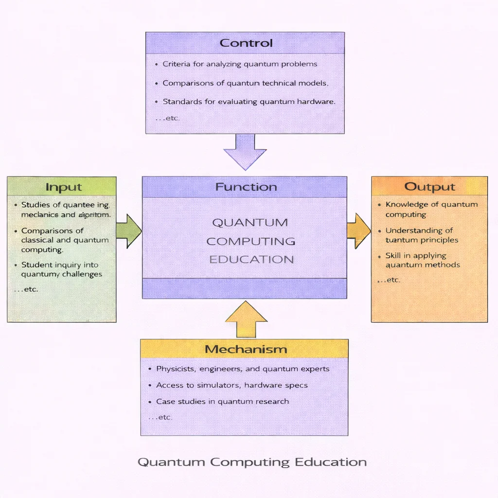
Quantum computing education is not simply the delivery of abstract information—it is the disciplined transformation of curiosity into structured, verifiable physical and computational understanding. Learners begin with fundamental inputs: the state space of quantum bits (qubits), linear superposition, unitary transformations, projective measurement, and the mathematical contrast between classical boolean logic and complex Hilbert state spaces. Governed by formal controls—the postulates of quantum mechanics, error-propagation limits, and decoherence bounds—students approach quantum computation not as speculative theory, but as an engineered system that can be mathematically formulated, simulated, and benchmarked against classical limits.
Quantum computing represents a fundamental departure from classical Von Neumann computational architecture. By exploiting quantum mechanical phenomena—specifically state superposition, phase interference, and non-local entanglement—quantum algorithms solve specific classes of high-dimensional problems that are intractable for classical supercomputers. Its advancement is deeply interconnected with artificial intelligence and machine learning, where quantum algorithms promise exponential and polynomial speedups for continuous optimization, kernel evaluations, and probabilistic sampling. As a core frontier in emerging technologies, quantum computing also accelerates innovations across biotechnology and data science and analytics.
Beyond computer science, quantum mechanics transforms engineering disciplines. In energy storage and renewable systems, quantum simulation models atomic-scale catalytic reactions and solid-state battery interfaces. In environmental engineering, quantum-enhanced linear solvers model atmospheric fluid dynamics with high resolution. Furthermore, quantum communications and Quantum Key Distribution (QKD) provide physically secure channels for smart IoT infrastructure and industrial Industry 4.0 networks.

Core Pillars of Quantum Information: Child Modules
Mastering quantum computing requires building from individual two-level quantum systems up to multi-qubit entangled circuits. Explore the four specialized child modules comprising this sub-hub:
1. Quantum Bits (Qubits) →
The fundamental unit of quantum information. Explores physical implementations (superconducting transmons, trapped ions), the Bloch sphere geometric representation, and projective state measurement.
Destination URL: https://prep4uni.online/stem/emerging-technologies/quantum-computing/qubits/2. Quantum Superposition →
Linear combinations of orthogonal basis states. Investigates wave function mechanics, probability amplitude normalization, constructive and destructive interference, and quantum parallelism.
Destination URL: https://prep4uni.online/stem/emerging-technologies/quantum-computing/quantum-superposition/3. Quantum Entanglement →
Non-separable composite multi-qubit states. Examines the four canonical Bell states, the Einstein-Podolsky-Rosen (EPR) paradox, Bell's inequality tests, and quantum teleportation protocols.
Destination URL: https://prep4uni.online/stem/emerging-technologies/quantum-computing/quantum-entanglement/4. Quantum Gates and Circuits →
Unitary matrix transformations on Hilbert state spaces. Analyzes single-qubit gates (Pauli-X, Y, Z, Hadamard, Phase) and multi-qubit entangling gates (CNOT, Toffoli, SWAP) for algorithm compilation.
Destination URL: https://prep4uni.online/stem/emerging-technologies/quantum-computing/quantum-gates-and-circuits/Mathematical Foundations of Quantum States
A single qubit exists as a normalized state vector in a two-dimensional complex Hilbert space (\(\mathcal{H}_2\)). Expressed in Dirac bra-ket notation relative to the orthonormal computational basis states \(\{|0\rangle, |1\rangle\}\):
Qubit State Vector Formulation:
$$|\psi\rangle = \alpha|0\rangle + \beta|1\rangle \quad \text{where } \alpha, \beta \in \mathbb{C}$$The complex probability amplitudes \(\alpha\) and \(\beta\) define the coordinate projections along the computational basis axes.
According to the Born rule, projective measurement of \(|\psi\rangle\) collapses the state vector into classical outcome \(0\) with probability \(P(0) = |\alpha|^2\) or outcome \(1\) with probability \(P(1) = |\beta|^2\). Because measurement outcomes form a complete probability distribution, the state vector must satisfy the strict normalization constraint:
Normalization Constraint:
$$\langle\psi|\psi\rangle = |\alpha|^2 + |\beta|^2 = 1$$Ensures the sum of all mutually exclusive measurement probabilities equals unity (\(100\%\)).
When scaling to an \(n\)-qubit register, the composite state space expands via the tensor product (\(\mathcal{H}_{2^n} = \mathcal{H}_2^{\otimes n}\)):
$$|\Psi\rangle = \sum_{x=0}^{2^n - 1} c_x |x\rangle \quad \text{subject to} \quad \sum_{x=0}^{2^n - 1} |c_x|^2 = 1$$An \(n\)-qubit quantum processor simultaneously maintains \(2^n\) complex probability amplitudes, producing an exponential expansion of computational state space that underpins quantum computational advantages.
Applied Domains: Quantum Advantage in Engineering & Science
Quantum algorithms offer significant improvements in computational complexity across specialized computational classes:
| Application Domain | Algorithmic Mechanism | Industrial / Scientific Impact |
|---|---|---|
| Molecular Simulation & Drug Discovery | Variational Quantum Eigensolver (VQE) and Quantum Phase Estimation (QPE) mapping electronic Hamiltonians directly onto physical qubit registers. | Simulating nitrogenase FeMoco active sites for industrial fertilizer synthesis and de novo oncology drug ligand docking. |
| Post-Quantum Cryptography & Security | Shor’s algorithm achieving polynomial-time prime factorization (\(\mathcal{O}((\log N)^3)\)), driving the adoption of lattice-based post-quantum cryptography (PQC). | Transitioning global banking, defense, and public-key infrastructure to NIST-standardized quantum-resistant algorithms. |
| Combinatorial Optimization & Logistics | Quantum Approximate Optimization Algorithm (QAOA) and quantum annealing exploring complex energy landscapes. | Fleet route optimization, air traffic congestion minimization, and multi-asset financial portfolio rebalancing. |
| Quantum Machine Learning (QML) | Harrow-Hassidim-Lloyd (HHL) algorithm accelerating matrix inversion (\(A\mathbf{x}=\mathbf{b}\)) exponentially from \(\mathcal{O}(N^3)\) to \(\mathcal{O}(\log(N))\). | High-dimensional support vector machines, anomaly detection in financial networks, and generative quantum models. |
Interactive Quantum Circuit Fidelity & Noise Simulator
Simulate how physical single-gate fidelity and environmental decoherence affect overall quantum circuit fidelity as circuit depth increases:
Interactive Review Checkpoints
Click each question to toggle the detailed answer key and verify your conceptual understanding:
Review Checkpoint 1: How does quantum measurement alter the state vector of a qubit?
Review Checkpoint 2: What makes Grover's algorithm computationally advantageous over classical searching?
Frequently Asked Questions on Quantum Computing
1. What is quantum computing in fundamental engineering terms?
Quantum computing is a computational paradigm that processes information using quantum two-level systems (qubits) governed by the laws of quantum mechanics. Unlike classical computers restricted to binary bits (\(0\) or \(1\)), quantum processors utilize linear combinations of states, constructive/destructive wave interference, and entanglement to evaluate complex state spaces in parallel.
2. What physical mechanisms cause quantum decoherence?
Decoherence occurs when physical qubits interact with their thermal, electromagnetic, or material environment. Background blackbody radiation, stray magnetic fluctuations, and material dielectric loss cause relative phase randomization (phase relaxation time, \(T_2\)) and spontaneous energy dissipation to the ground state (longitudinal relaxation time, \(T_1\)), destroying quantum information.
3. What does Noisy Intermediate-Scale Quantum (NISQ) mean?
NISQ describes current-generation quantum hardware containing roughly 50 to 1,000 physical qubits that lack fault-tolerant quantum error correction. Because gate fidelities are imperfect (\(\sim 99.0\% - 99.9\%\)), cumulative errors restrict circuit depth, making NISQ systems suitable primarily for hybrid classical-quantum algorithms like VQE and QAOA.
Comprehensive Quantum Practice Suite
Part A: Core Knowledge & Foundational Review Questions
1. Contrast an 8-bit classical register with an 8-qubit quantum register.
2. Why doesn't quantum entanglement permit faster-than-light communication?
3. Explain the foundational concept of Quantum Error Correction (QEC).
Part B: Thought-Provoking & Analytical Scenarios
1. What is the "Harvest Now, Decrypt Later" cryptographic security threat?
2. What physical and cryogenic bottlenecks limit quantum hardware scaling?
Part C: Quantitative Calculations & Step-by-Step Solutions
Problem 1: Register Hilbert Space Dimensionality Sizing
Scenario: A quantum processor register contains \(n = 8\) entangled physical qubits. Determine the total number of orthogonal basis states that can be maintained simultaneously in linear superposition, and compute the base-2 logarithm of that state dimension.
Step-by-Step Derivation:
$$ \begin{aligned} D &= 2^n = 2^8 = 256 \text{ basis states} \\ \log_2(D) &= \log_2(256) = 8 \end{aligned} $$Answer & Conclusion: The 8-qubit register simultaneously spans a Hilbert space of exactly 256 orthogonal states.
Problem 2: Exponential Computational Operation Scaling
Scenario: A brute-force state simulation scales as \(\mathcal{O}(2^n)\). A 10-qubit system requires \(2^{10} = 1{,}024\) operations. Calculate the operations required for an expanded register of \(n = 15\) qubits.
Step-by-Step Derivation:
$$ \begin{aligned} N_{15} &= 2^{15} = 2^{10} \times 2^5 = 1{,}024 \times 32 = 32{,}768 \text{ operations} \end{aligned} $$Answer & Conclusion: Scaling the register by 5 qubits increases computational requirements to \(32{,}768 \text{ operations}\).
Problem 3: Born Rule Modulus Squaring and Probability Extraction
Scenario: A qubit's probability amplitude for basis state \(|1\rangle\) is given by the complex scalar \(c_1 = 0.30 + 0.40i\). Using the Born rule, calculate the modulus \(|c_1|\) and the probability of measuring state \(|1\rangle\).
Step-by-Step Derivation:
$$ \begin{aligned} |c_1| &= \sqrt{\text{Re}(c_1)^2 + \text{Im}(c_1)^2} = \sqrt{0.30^2 + 0.40^2} = \sqrt{0.09 + 0.16} = \sqrt{0.25} = 0.50 \\ P(1) &= |c_1|^2 = (0.50)^2 = 0.25 = 25.0\% \end{aligned} $$Answer & Conclusion: The measurement probability for basis state \(|1\rangle\) is exactly \(0.25\) (or \(25.0\%\)).
Problem 4: Cumulative Circuit Fidelity Across Gate Depth
Scenario: A quantum circuit consists of a sequence of \(N = 50\) gates. Each gate operates with an average single-gate fidelity of \(F_g = 98.0\%\) (\(0.98\)). Assuming independent errors without error correction, compute the cumulative circuit fidelity.
Step-by-Step Derivation:
$$ \begin{aligned} F_{\text{total}} &= (F_g)^N = (0.98)^{50} \\ \ln(F_{\text{total}}) &= 50 \times \ln(0.98) \approx 50 \times (-0.0202027) \approx -1.010135 \\ F_{\text{total}} &= e^{-1.010135} \approx 0.36417 \end{aligned} $$Answer & Conclusion: Cumulative circuit fidelity decreases to approximately \(36.42\%\), showing how errors compound with circuit depth.
Problem 5: Quadratic Search Complexity Reduction
Scenario: An unsorted database contains \(N = 1{,}000{,}000\) records. A classical linear search takes an average of \(N/2 = 500{,}000\) operations. Grover’s algorithm achieves a quadratic speedup of \(\mathcal{O}(\sqrt{N})\). Compute the quantum query operations required.
Step-by-Step Derivation:
$$ \begin{aligned} C_{\text{quantum}} &\approx \sqrt{N} = \sqrt{1{,}000{,}000} = 1{,}000 \text{ oracle queries} \\ \text{Speedup Ratio} &= \frac{C_{\text{classical}}}{C_{\text{quantum}}} = \frac{500{,}000}{1{,}000} = 500\times \end{aligned} $$Answer & Conclusion: Grover’s algorithm resolves the target in approximately \(1{,}000 \text{ operations}\), delivering a \(500\times\) speedup.
Problem 6: Quantum Error Correction Reduction Factor
Scenario: An experimental logical qubit architecture reduces a raw physical error rate of \(\epsilon_0 = 5.0\%\) (\(0.05\)) by a factor of \(10\times\). Calculate the effective logical error rate.
Step-by-Step Derivation:
$$ \begin{aligned} \epsilon_{\text{logical}} &= \frac{\epsilon_0}{10} = \frac{0.05}{10} = 0.005 = 0.50\% \end{aligned} $$Answer & Conclusion: The effective logical error rate is reduced to \(0.50\%\).
Problem 7: Maximum Coherent Gate Operations Calculation
Scenario: A superconducting transmon qubit exhibits a coherence time of \(T_{\text{coh}} = 100.0 \ \mu\text{s}\). The duration of a single microwave-driven control gate is \(t_{\text{gate}} = 10.0 \text{ ns}\). Determine the theoretical maximum number of sequential gate operations that can execute before coherence is lost.
Step-by-Step Derivation:
$$ \begin{aligned} T_{\text{coh}} &= 100.0 \ \mu\text{s} = 100{,}000.0 \text{ ns} \\ N_{\text{max}} &= \frac{T_{\text{coh}}}{t_{\text{gate}}} = \frac{100{,}000.0 \text{ ns}}{10.0 \text{ ns}} = 10{,}000 \text{ operations} \end{aligned} $$Answer & Conclusion: The processor can execute up to \(10{,}000 \text{ gate operations}\) within its coherence window.
Problem 8: Repeated Sampling and Success Confidence Thresholds
Scenario: A randomized quantum algorithm has a success probability of \(p = 0.70\) on any single run. Determine the minimum number of independent circuit runs (\(n\)) required to achieve an overall success probability of at least \(95.0\%\) (\(P_{\text{succ}} \ge 0.95\)).
Step-by-Step Derivation:
$$ \begin{aligned} P_{\text{fail, single}} &= 1 - p = 1 - 0.70 = 0.30 \\ P_{\text{fail, total}} &= (0.30)^n \le 1 - 0.95 = 0.05 \\ n \times \ln(0.30) &\le \ln(0.05) \\ n \times (-1.20397) &\le -2.99573 \implies n \ge \frac{-2.99573}{-1.20397} \approx 2.488 \end{aligned} $$Answer & Conclusion: Rounding up to the nearest integer, a minimum of \(n = 3 \text{ runs}\) is required to guarantee a \(\ge 95\%\) success rate.
Problem 9: Energy Dissipation Per Quantum Logic Gate
Scenario: A dilution refrigerator cooling stage draws an effective power of \(P = 150.0 \text{ W}\) while the quantum chip executes \(R = 10^{12} \text{ gate operations per second}\). Calculate the average energy consumed per operation in Joules.
Step-by-Step Derivation:
$$ \begin{aligned} E_{\text{op}} &= \frac{P}{R} = \frac{150.0 \text{ J}\cdot\text{s}^{-1}}{10^{12} \text{ operations}\cdot\text{s}^{-1}} = 1.50 \times 10^{-10} \text{ J/operation} \end{aligned} $$Answer & Conclusion: The system dissipates approximately \(1.50 \times 10^{-10} \text{ Joules}\) (or \(0.15 \text{ nJ}\)) per operation.
Problem 10: Percentage Reduction in Quantum Error Rates
Scenario: Dynamical decoupling pulses reduce a two-qubit gate error rate from \(\epsilon_1 = 5.0\%\) down to \(\epsilon_2 = 1.0\%\). Determine the absolute reduction and the relative percentage reduction.
Step-by-Step Derivation:
$$ \begin{aligned} \Delta \epsilon &= 5.0\% - 1.0\% = 4.0\% \text{ absolute} \\ \text{Relative Reduction} &= \left( \frac{\Delta \epsilon}{\epsilon_1} \right) \times 100\% = \left( \frac{4.0\%}{5.0\%} \right) \times 100\% = 80.0\% \end{aligned} $$Answer & Conclusion: The pulse sequences achieve an \(80.0\%\) relative reduction in gate error rate.
Problem 11: High-Throughput State Evaluation Rates
Scenario: A classical state-vector simulator executes \(f = 10.0 \text{ iterations/s}\). Each iteration models a register of \(2^{20}\) state amplitudes. Calculate the total number of state vector evaluations completed per minute.
Step-by-Step Derivation:
$$ \begin{aligned} 2^{20} &= 1{,}048{,}576 \text{ amplitudes per iteration} \\ R_{\text{sec}} &= 1{,}048{,}576 \times 10.0 = 10{,}485{,}760 \text{ evaluations/s} \\ R_{\text{min}} &= 10{,}485{,}760 \text{ evals/s} \times 60.0 \text{ s} = 629{,}145{,}600 \text{ evaluations/min} \approx 6.29 \times 10^8 \end{aligned} $$Answer & Conclusion: The simulator performs approximately \(6.29 \times 10^8 \text{ evaluations per minute}\).
Problem 12: Large-Scale Complexity Reduction Comparison
Scenario: An unindexed scientific database contains \(N = 10^8\) entries. Compare the computational steps required by a classical linear search versus Grover's quantum search.
Step-by-Step Derivation:
$$ \begin{aligned} S_{\text{classical}} &= N = 10^8 = 100{,}000{,}000 \text{ operations} \\ S_{\text{quantum}} &= \sqrt{N} = \sqrt{10^8} = 10^4 = 10{,}000 \text{ operations} \\ \text{Reduction Factor} &= \frac{10^8}{10^4} = 10^4 = 10{,}000\times \end{aligned} $$Answer & Conclusion: The quantum search reduces the operation count by a factor of \(10{,}000\times\).
Quantum Computing: Summary & Learning Wrap-Up
Quantum computing transitions information theory from binary logic into linear transformations over complex Hilbert spaces. By linking the foundational child topics—Qubits, Superposition, Entanglement, and Unitary Gate Circuits—students build an end-to-end understanding of how quantum processors achieve computational advantages while managing decoherence and noise. Mastering these concepts prepares learners to lead advancements across post-quantum cryptography, molecular simulation, and scientific computing.