
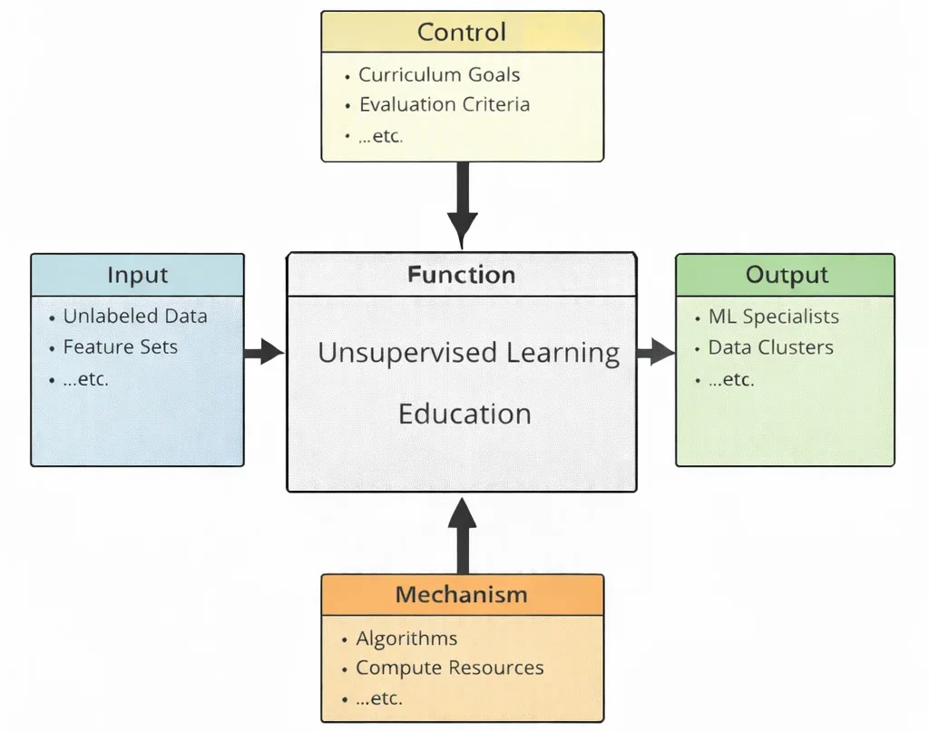

Artificial Intelligence & Machine Learning Topic Hub
Core Concepts of Unsupervised Learning
Absence of Labels
Unlike supervised learning, where each instance is paired with a known target, unsupervised learning has no ground-truth “answer key.” Models rely entirely on input feature vectors to detect commonalities, differences, and statistical relationships.
Discovery of Hidden Structures
Without explicit guidance, models reveal underlying pattern manifolds, naturally occurring clusters, or informative low-dimensional subspaces that condense complex data distributions.
Adaptability & Exploratory Analysis
Unsupervised methods serve as an indispensable first step in exploratory data analysis (EDA), helping data scientists characterize raw, unannotated datasets prior to downstream predictive modeling.
Common Techniques in Unsupervised Learning
1. Clustering
Partitions data points into cohesive groups (clusters) such that intra-cluster similarity is maximized while inter-cluster similarity is minimized:
- Customer Segmentation: Groups users based on purchasing behavior, frequency, and demographic features for targeted marketing.
- Document Grouping: Clusters unstructured text corpora into thematic topics without pre-existing classification taxonomies.
- Primary Algorithms: K-Means (fast, centroid-based), Hierarchical Clustering (nested dendrogram trees), and DBSCAN (density-based, shape-agnostic clustering).
2. Dimensionality Reduction
Transforms high-dimensional feature spaces into lower-dimensional representations while preserving maximum variance or local geometric structure:
- Principal Component Analysis (PCA): Linear orthogonal transformation identifying directions of maximum variance.
- t-SNE & UMAP: Non-linear manifold learning techniques preserving local neighborhood topology for low-dimensional visualization.
Evaluation & Validation for Unsupervised Learning
Internal Validation Metrics
- Silhouette Score (-1.0 to +1.0): Quantifies intra-cluster cohesion a versus nearest-cluster separation b:
$$\text{Silhouette} = \frac{b – a}{\max(a, b)}$$
- Davies–Bouldin Index (≥ 0): Evaluates the average similarity ratio of each cluster with its most similar counterpart. Lower values indicate superior cluster separation.
- Calinski–Harabasz Index: Measures the ratio of between-cluster dispersion to within-cluster dispersion. Higher values denote denser, well-separated clusters.
External Validation Metrics (Reference Benchmarks)
- Adjusted Rand Index (ARI): Measures label agreement between discovered clusters and reference ground truth, corrected for chance (-1.0 to +1.0).
- Normalized Mutual Information (NMI): Normalizes mutual information between cluster assignments and reference classes to a [0.0, 1.0] interval.
Cluster Evaluation Recipe
import numpy as np
from sklearn.cluster import KMeans
from sklearn.metrics import silhouette_score, davies_bouldin_score, calinski_harabasz_score

def evaluate_clustering_quality(X: np.ndarray, labels: np.ndarray) -> dict:
    """Computes comprehensive internal validation metrics for cluster evaluation."""
    return {
        "silhouette": float(silhouette_score(X, labels)),
        "davies_bouldin": float(davies_bouldin_score(X, labels)),
        "calinski_harabasz": float(calinski_harabasz_score(X, labels))
    }

def sweep_optimal_k(X: np.ndarray, k_min: int = 2, k_max: int = 10) -> tuple:
    """Sweeps cluster count k to identify optimal Silhouette score peak."""
    scores = []
    for k in range(k_min, k_max + 1):
        km = KMeans(n_clusters=k, n_init=10, random_state=42).fit(X)
        s = silhouette_score(X, km.labels_)
        scores.append((k, s))
    best_k, best_s = max(scores, key=lambda t: t[1])
    return best_k, scores
Leakage-Safe Pipelines for Unsupervised → Supervised Workflows
from sklearn.compose import ColumnTransformer
from sklearn.pipeline import Pipeline, FeatureUnion
from sklearn.preprocessing import StandardScaler, OneHotEncoder
from sklearn.decomposition import PCA
from sklearn.cluster import KMeans
from sklearn.linear_model import LogisticRegression
from sklearn.model_selection import StratifiedKFold, cross_val_score

num_cols = ["age", "income", "tenure"]
cat_cols = ["city", "segment"]

preprocessor = ColumnTransformer([
    ("num", StandardScaler(), num_cols),
    ("cat", OneHotEncoder(handle_unknown="ignore"), cat_cols)
])

# Combine linear PCA components with non-linear KMeans distance vectors
unsupervised_features = FeatureUnion([
    ("pca", PCA(n_components=12, random_state=42)),
    ("kmeans", KMeans(n_clusters=8, n_init=10, random_state=42))
])

full_pipeline = Pipeline([
    ("pre", preprocessor),
    ("unsup", unsupervised_features),
    ("clf", LogisticRegression(max_iter=2000))
])

cv = StratifiedKFold(n_splits=5, shuffle=True, random_state=42)
scores = cross_val_score(full_pipeline, X, y, cv=cv, scoring="roc_auc")
print(f"Leakage-Safe CV ROC-AUC: {scores.mean():.4f} +/- {scores.std():.4f}")
Interpreting Clusters: Profiles, Exemplars & Drift Monitoring
1. Cluster Profiling & Exemplar Extraction
import pandas as pd
import numpy as np
from sklearn.metrics import pairwise_distances_argmin_min

def build_cluster_profiles(df_features: pd.DataFrame, cluster_labels: np.ndarray) -> pd.DataFrame:
    """Generates statistical profile summary table per discovered cluster."""
    df = df_features.copy()
    df["cluster"] = cluster_labels
    return df.groupby("cluster").agg(["mean", "median", "std"])

def get_cluster_exemplars(X: np.ndarray, labels: np.ndarray, cluster_centers: np.ndarray, k_top: int = 3) -> dict:
    """Finds indices of data instances closest to each cluster centroid."""
    exemplars = {}
    for c_id in range(cluster_centers.shape[0]):
        cluster_indices = np.where(labels == c_id)[0]
        _, distances = pairwise_distances_argmin_min(X[cluster_indices], cluster_centers[c_id].reshape(1, -1))
        top_k = cluster_indices[np.argsort(distances.ravel())[:k_top]]
        exemplars[c_id] = top_k.tolist()
    return exemplars
2. Production Drift Tracking Utilities
from scipy.spatial.distance import jensenshannon

def compute_centroid_shift(baseline_centers: np.ndarray, production_centers: np.ndarray) -> np.ndarray:
    """Computes per-cluster Euclidean centroid movement between training and production."""
    return np.linalg.norm(baseline_centers - production_centers, axis=1)

def compute_js_divergence(p_baseline: np.ndarray, q_production: np.ndarray) -> float:
    """Computes Jensen-Shannon distance for cluster population proportion shifts."""
    p = np.clip(p_baseline, 1e-12, 1.0); p /= p.sum()
    q = np.clip(q_production, 1e-12, 1.0); q /= q.sum()
    return float(jensenshannon(p, q))
Dimensionality Reduction Cheat-Sheet (PCA • UMAP • t-SNE)
| Algorithm | Mathematical Nature | Preserved Structure | Primary Operational Use Case |
|---|---|---|---|
| PCA | Linear orthogonal projection | Global variance directions | Feature compression, noise reduction, linear baselines |
| UMAP | Non-linear manifold learning | Local & global manifold graph topology | Pre-clustering embeddings, high-fidelity visualization |
| t-SNE | Non-linear probabilistic mapping | Local point-wise neighborhood distances | 2D/3D visual cluster exploration (Not for features) |
Anomaly Detection in Practice
Detector Selection
- Isolation Forest: Tree-ensemble partitioning that isolates anomalies near tree roots. Excellent tabular default.
- Local Outlier Factor (LOF): Compares local density of a sample against its k-nearest neighbors.
- One-Class SVM: Fits a tight support boundary around normal training distributions in high-dimensional space.
Isolation Forest Implementation
import numpy as np
from sklearn.ensemble import IsolationForest
from sklearn.pipeline import Pipeline
from sklearn.preprocessing import StandardScaler

anomaly_pipeline = Pipeline([
    ("scaler", StandardScaler()),
    ("iso", IsolationForest(n_estimators=300, contamination=0.01, random_state=42))
])

# Fit strictly on clean training normal distribution
anomaly_pipeline.fit(X_train)

# Raw scores: lower negative values indicate higher anomaly severity
raw_scores = anomaly_pipeline.decision_function(X_val)
anomaly_rankings = -raw_scores  # Invert so higher score = higher risk
Self-Supervised Learning (SSL) for Representation Learning
Core Families
- Contrastive Learning (e.g., SimCLR, MoCo): Maximizes representation agreement between differently augmented views of the same instance using InfoNCE loss while pulling distinct items apart.
- Masked Pretext Modeling (e.g., BERT MLM, Masked Autoencoders): Hides random tokens or image patches and trains models to reconstruct original inputs.
Linear-Probe Evaluation (Fast Check for SSL/Embeddings)
from sklearn.linear_model import LogisticRegression
from sklearn.metrics import f1_score

# Freeze encoder embeddings (E_train, E_val) and fit linear classifier
probe = LogisticRegression(max_iter=2000)
probe.fit(E_train, y_train_small)

val_predictions = probe.predict(E_val)
probe_f1 = f1_score(y_val_small, val_predictions, average="macro")
print(f"Linear Probe Validation Macro F1: {probe_f1:.4f}")
Mini Playbook & Production Retraining Cron
Operational Workflow
- Clean data & define leakage-safe pipeline (Scalers + Encoders fit on Train split).
- Compress input dimensions using PCA or UMAP embeddings.
- Apply K-Means or DBSCAN clustering over low-dimensional embeddings.
- Validate cluster separation using Silhouette scores and profile centroids.
- Deploy monitoring cron jobs to alert on centroid shift and population mix drift.
Nightly Monitoring Cron Job Script
# Nightly Unsupervised Health Audit Skeleton
import json
import numpy as np
from sklearn.metrics import silhouette_score

def audit_production_clusters(live_embeddings: np.ndarray, live_labels: np.ndarray, baseline_centers: np.ndarray) -> dict:
    """Executes automated nightly cluster health and drift check."""
    current_sil = float(silhouette_score(live_embeddings, live_labels))

    # Compute shift across active cluster centroids
    live_centers = np.array([live_embeddings[live_labels == k].mean(axis=0) for k in np.unique(live_labels)])
    max_drift = float(np.max(np.linalg.norm(baseline_centers - live_centers, axis=1)))

    alerts = []
    if current_sil < 0.25:
        alerts.append("WARNING: Silhouette quality dropped below 0.25 threshold!")
    if max_drift > 0.50:
        alerts.append("ALERT: Centroid position drift exceeded 0.50 L2 threshold!")

    return {"silhouette": current_sil, "max_centroid_drift": max_drift, "alerts": alerts}
Key Terms Glossary
- Unsupervised Learning
- Machine learning paradigm extracting intrinsic structure, clusters, or representations from unlabeled data.
- Silhouette Score
- Internal metric measuring cluster compactness versus separation on a [-1.0, +1.0] scale.
- Principal Component Analysis (PCA)
- Linear orthogonal dimensionality reduction technique maximizing variance along uncorrelated principal components.
- Isolation Forest
- Tree-based anomaly detection algorithm isolating outliers via randomized recursive attribute partitioning.
- Jensen-Shannon Divergence
- Symmetric statistical measure quantifying probability distribution divergence between baseline and live features.
Unsupervised Learning: Frequently Asked Questions
What is unsupervised learning, and how is it different from supervised learning?
Unsupervised learning trains models on unlabeled data to discover hidden patterns, groupings, or representations. Supervised learning uses labeled target pairs to learn an explicit mapping from inputs to known outputs.
What are the primary types of unsupervised learning algorithms?
The primary categories are clustering (K-Means, DBSCAN), dimensionality reduction (PCA, UMAP), anomaly detection (Isolation Forest, LOF), and density estimation.
How do you evaluate clustering quality without ground-truth labels?
Use internal validation metrics such as Silhouette score, Davies-Bouldin index, and Calinski-Harabasz score, alongside cluster stability tests across random seeds.
Why is feature scaling essential before applying PCA or K-Means?
Distance-based algorithms and variance-maximizing projections are highly sensitive to raw feature scales. Unscaled features with large numerical ranges will dominate distance calculations and principal component directions.
End-of-Page Exercises & Assessment
Part 1: Review Questions
Q1: Define unsupervised learning and state its three core application domains.
Answer: Unsupervised learning discovers natural structure in unlabeled data without target guidance. Its primary application domains are clustering, dimensionality reduction, and anomaly detection.
Q2: Explain the mathematical distinction between the Silhouette Score and the Davies-Bouldin Index.
Answer: Silhouette score measures intra-cluster cohesion relative to nearest-cluster separation on a [-1.0, +1.0] bounded scale (higher is better). Davies-Bouldin index measures average similarity ratios between clusters (lower is better, 0 indicates optimal separation).
Q3: How does DBSCAN handle noise and arbitrary cluster geometries compared to K-Means?
Answer: K-Means enforces spherical clusters and assigns every point to a centroid. DBSCAN groups points based on local density parameters (eps, min_samples), discovering arbitrary non-spherical shapes while explicitly categorizing low-density points as noise outliers.
Q4: What risk arises when performing PCA before cross-validation splitting?
Answer: Data leakage. Fitting PCA across all samples exposes training models to variance statistics from validation/testing subsets, yielding overly optimistic performance estimates.
Part 2: Thought-Provoking Questions
Q1: High-Dimensional Distance Concentration in K-Means Clustering
Scenario: An engineer applies K-Means clustering directly to raw 1,024-dimensional image embeddings. The Silhouette score drops near 0.00, and cluster centroids collapse toward identical pairwise distances.
Analysis: The algorithm suffered from the Curse of Dimensionality (distance concentration phenomenon), where pairwise Euclidean distances become uniformly distant in high dimensions. The resolution is pre-compressing dimensions to 10–32 components using UMAP or linear PCA prior to clustering.
Q2: Silent Production Failure in Anomaly Detection Engines
Scenario: An Isolation Forest model deployed for fraud detection generates zero security alerts for two weeks despite high transaction volumes.
Analysis: The system suffered from Data Drift or contamination parameter miscalibration. Input feature distributions shifted, causing raw decision scores to remain above the fixed alert threshold. Implementing nightly Jensen-Shannon divergence tracking and dynamic percentile thresholding resolves this failure mode.
Part 3: Numerical Engineering Problems
Problem 1: Euclidean Distance Calculation Between High-Dimensional Points
Question: Given two 3D vector points A = (2.0, -1.0, 3.0) and B = (5.0, 1.0, 0.0):
1. Calculate coordinate differences (B – A).
2. Calculate the squared Euclidean distance.
3. Calculate the exact Euclidean distance.
Step-by-step Solution:
1. Differences:
• Δx = 5.0 – 2.0 = 3.0
• Δy = 1.0 – (-1.0) = 2.0
• Δz = 0.0 – 3.0 = -3.0
2. Squared Distance:
• d2 = (3.0)2 + (2.0)2 + (-3.0)2 = 9.0 + 4.0 + 9.0 = 22.0.
3. Euclidean Distance:
• d = √22.0 ≈ 4.6904.
Final Answer: Euclidean distance is approximately 4.6904.
Problem 2: Within-Cluster Sum of Squares (WCSS / SSE) Calculation
Question: A cluster centroid resides at C = (3.0, 4.0) with three assigned data instances: P1 = (2.0, 3.0), P2 = (3.0, 4.0), and P3 = (4.0, 5.0). Calculate total Within-Cluster Sum of Squares (WCSS).
Step-by-step Solution:
1. Squared distance for P1:
• (2.0 – 3.0)2 + (3.0 – 4.0)2 = (-1.0)2 + (-1.0)2 = 1.0 + 1.0 = 2.0.
2. Squared distance for P2:
• (3.0 – 3.0)2 + (4.0 – 4.0)2 = 0.0.
3. Squared distance for P3:
• (4.0 – 3.0)2 + (5.0 – 4.0)2 = (1.0)2 + (1.0)2 = 1.0 + 1.0 = 2.0.
4. Sum WCSS:
• WCSS = 2.0 + 0.0 + 2.0 = 4.0.
Final Answer: Total WCSS is 4.0.
Problem 3: Silhouette Score Calculation
Question: For a single sample, average intra-cluster distance a = 2.50, and nearest inter-cluster distance b = 4.00. Compute the Silhouette score.
Step-by-step Solution:
1. Silhouette Formula:
• s = (b – a) / max(a, b)
• s = (4.00 – 2.50) / max(2.50, 4.00) = 1.50 / 4.00 = 0.3750.
Final Answer: Silhouette score is 0.3750.
Problem 4: PCA Explained Variance Ratio Calculation
Question: A 3D feature covariance matrix yields eigenvalues λ1 = 5.0, λ2 = 3.0, and λ3 = 2.0. Calculate the proportion of total variance explained by the first principal component.
Step-by-step Solution:
1. Total Variance = 5.0 + 3.0 + 2.0 = 10.0.
2. First Component Ratio = λ1 / Total = 5.0 / 10.0 = 0.5000 (50.0%).
Final Answer: The first principal component explains 50.0% of total variance.
Closing Summary & Next Steps
AI Sub-Cluster Links
-
Supervised Learning
Explore training models using explicit labels, loss functions, and classification/regression pipelines. -
Deep Learning
Discover multi-layer neural networks, autoencoders, and self-supervised representations. -
MLOps & AI Infrastructure
Learn about CI/CD pipelines, feature stores, and automated production telemetry monitoring. -
Artificial Intelligence Hub
Return to the main AI overview hub covering core machine learning paradigms and applications.
External References
- Scikit-Learn Clustering Documentation – Official technical documentation on clustering metrics and pipelines.
- UMAP: Uniform Manifold Approximation and Projection – Technical documentation for UMAP embeddings.