Prepare for University Studies & Career Advancement

Signal Processing

Signal Processing Education trains learners to turn messy measurements into meaning. Starting with real-world signals—often noisy, incomplete, and distorted—students learn how to model, sample, filter, and analyze data so that important patterns survive while distractions fade. The governing constraints (design standards, accuracy targets, bandwidth limits, and safety expectations) shape what “good processing” actually means in practice, not just in theory. Using tools such as simulation software, algorithm libraries, lab instruments, and embedded platforms, learners repeatedly test ideas against reality—tuning filters, comparing methods, and validating results. By the end, the payoff is tangible: the ability to produce trustworthy analyses and signal-driven outputs that support decisions, diagnostics, detection, communication, and control in systems people rely on.

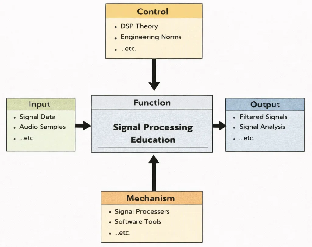
Figure 1: IDEF0 view of Signal Processing Education: how raw signals are transformed into reliable information and actionable decisions.

This IDEF0 diagram summarizes the educational “process flow” of Signal Processing Education. On the left, typical inputs include time-series signals and sampled data streams; from above, controls represent design requirements such as performance targets, safety constraints, and methodological standards. At the bottom, mechanisms highlight the enabling resources—software tools, algorithms, lab instruments, and computing platforms that students use to test ideas and validate results. The outputs on the right reflect what learners can produce after training: denoised signals, extracted features, spectral/temporal analyses, and signal-driven systems that support communication, sensing, diagnostics, and automation.

Signal processing is the backbone of modern technology, enabling machines to analyze, interpret, and respond to data from the real world. It is pivotal in applications such as Robotics and Automation in E&E, where real-time processing of sensor inputs allows autonomous systems to make intelligent decisions. From managing climate systems to powering smart cities, signal processing is also deeply embedded in Environmental Engineering, especially in systems that monitor pollutants or optimize energy consumption.

In air quality monitoring, for instance, signal processing helps transform raw sensor outputs into actionable insights, supporting domains like Air Quality Engineering and Climate Change Mitigation and Adaptation. The ability to interpret environmental signals supports Ecological Engineering efforts and empowers large-scale Environmental Monitoring and Data Analysis. This data processing is also essential for evaluating policy effectiveness in Environmental Policy and Management.

Smart buildings rely on data-rich systems supported by signal processing to dynamically adapt lighting, HVAC, and energy usage, a critical aspect of Green Building and Sustainable Design. Moreover, in areas such as Industrial Ecology and Circular Economy and Renewable Energy Systems Engineering, signal processing technologies help optimize system efficiency and reduce waste. Applications extend to Waste Management Engineering and Water Resources Engineering, where signal feedback loops guide automation and system adjustments.

Signal processing also powers the digital transformation of manufacturing. It underpins technologies explored in Industrial and Manufacturing Technologies, such as Additive Manufacturing (3D Printing) and Advanced Materials and Manufacturing Technologies, where precision control of devices depends on accurate signal interpretation. Signal fidelity is critical for Computer-Integrated Manufacturing (CIM) and Digital Twin Technology, both of which rely on real-time system modeling.

Advances in signal processing are helping to improve Energy and Resource Efficiency in Manufacturing, and improving safety and productivity through attention to Human Factors and Ergonomics in Manufacturing. From quality assurance in Manufacturing Quality Control and Assurance to smart production frameworks like Smart Manufacturing and Industry 4.0, signal processing is central to intelligent systems. It even plays a role in optimizing operations under Lean Manufacturing and robotic coordination in Industrial Automation and Robotics, reflecting its foundational role in the future of innovation.

Interactive Digital Filter & Spectral Denoising Simulator

Simulate real-time digital filtering of a composite analog signal corrupted by high-frequency interference. Adjust signal fundamental frequency, noise amplitude, filter cutoff frequency, and filter topology to observe time-domain smoothing and frequency-domain attenuation.

Signal Frequency: 2.0 Hz

Noise Amplitude: 0.6 V

Filter Cutoff $f_c$: 4.0 Hz

Filter Architecture

Raw Input SNR: -- dB

Filtered Output SNR: -- dB

SNR Improvement: -- dB

Simulation runtime engine: Prep4Uni.Online Signal Processing Hub

Engineer in a futuristic control room analyzing signal waveforms and spectra on large holographic displays, with glowing frequency bars rising from an instrument console.

Figure 2: Signal Processing — turning raw waveforms into clean, usable information.

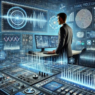
The image shows a high-tech signal analysis workspace where a specialist monitors multiple screens filled with waveforms, spectrogram-like patterns, and measurement panels. In the foreground, a sophisticated instrument console is overlaid with luminous “frequency bars,” visually suggesting spectral decomposition, filtering, and feature extraction. The surrounding displays hint at common signal-processing tasks such as noise reduction, frequency-domain analysis, pattern detection, and real-time monitoring—work that underpins communications, audio, radar/sonar, biomedical sensing, and control systems. Overall, the scene conveys signal processing as the disciplined art of converting complex, noisy data streams into meaningful, reliable insights.

Signal Processing: Curriculum Roadmap & Cluster Navigation

Electrical & Electronic Engineering Overview

Provides the broader system context where signals are generated, transmitted, and utilized.

Signal Processing (Current Page)

Analyses and transforms signals to extract information, reduce noise, and enable intelligent decision-making.

Communication Engineering

Relies on signal processing for encoding, modulation, transmission, and decoding of information.

Control Systems Engineering

Uses processed signals to regulate physical system behaviour through feedback mechanisms.

Instrumentation & Measurement

Captures raw physical signals that are conditioned and digitized to obtain calibrated measurements.

Embedded Systems & Microelectronics

Implements digital signal processing algorithms directly in real-time DSP, FPGA, and SoC hardware.

IoT & Smart Technologies

Applies edge signal processing to interpret and compress time-series sensor data across distributed nodes.

Robotics & Automation in EE

Filters and transforms multi-modal sensor inputs for robotic state estimation and trajectory planning.

Biomedical Electronics

Processes physiological signals like ECG, EEG, and EMG for real-time clinical diagnostics.

Quantum Electronics

Demodulates microwave dispersive readout tones and applies matched filtering to measure qubit states.

Power Systems Engineering

Detects grid waveform harmonics, symmetrical component imbalances, and transient fault arcs.

Renewable Energy & Storage

Processes stochastic weather datasets and battery impedance spectra for power forecasting and SoH estimation.

Electronics Engineering

Designs operational amplifier conditioning stages, active RC filters, and mixed-signal PCB interfaces.

Types of Signals

Analog SignalsAnalog signals are continuous waveforms that change smoothly over time and can take on an infinite number of values within a given range. These signals are typically found in natural phenomena and real-world measurements such as sound waves, light intensity, and temperature. Analog signals are characterized by their amplitude, frequency, and phase, and they require analog electronics—such as amplifiers, filters, and oscillators—for processing. Common applications of analog signals include audio systems, analog telephony, and instrumentation systems in scientific research. However, analog signals are prone to distortion and noise due to their continuous nature. As they travel over long distances or through multiple components, the signal may degrade, making amplification and filtering necessary to preserve signal integrity. To bridge the gap between the analog world and modern computation, analog-to-digital converters (ADCs) convert continuous analog inputs into discrete digital outputs.
Digital SignalsDigital signals are composed of discrete values—usually represented as binary numbers (0s and 1s). These signals result from sampling and quantizing analog signals, breaking the continuous waveform into a sequence of fixed intervals and corresponding numerical values. The robustness of digital signals against noise and degradation makes them the foundation of modern electronics and computing. Digital signals are integral to computers, smartphones, digital televisions, and networking systems. Their representation as binary data allows for precise control, easy error detection and correction, efficient compression, and integration with complex algorithms. Digital signal processing (DSP) is dedicated to analyzing and transforming digital signals using mathematical techniques. It plays a critical role in image processing, speech recognition, radar systems, and biomedical monitoring. While quantization introduces small errors, modern techniques minimize this loss through dithering and higher bit-depths.

Core Concepts in Signal Processing

Signal RepresentationSignals can be represented as functions of time (time domain), frequency (frequency domain), or space, depending on the application. In the time domain, signals reveal variations over duration, which is helpful in observing trends and fluctuations. In the frequency domain, transformations such as the Fourier Transform decompose a signal into its constituent sinusoidal components, which is crucial in communications, audio processing, and spectral analysis. The Laplace Transform, an extension of the Fourier Transform, is frequently employed in control systems to analyze system behavior and stability.
FilteringFilters play a pivotal role in extracting meaningful data from signals and reducing noise or unwanted spectral components. Depending on the application, filters are designed to operate in the time or frequency domain, using analog circuits or digital algorithms:
- Low-Pass Filters: Permit the transmission of signals below a specific cutoff frequency, effectively eliminating high-frequency noise.
- High-Pass Filters: Remove low-frequency content, often used in edge detection or to eliminate DC drift in instrumentation.
- Band-Pass Filters: Pass a band of frequencies while attenuating frequencies outside the range, isolating individual communication channels.
- Notch Filters: Precisely suppress a narrow frequency band, such as 50/60 Hz power line interference in biomedical recordings.
Modulation and DemodulationIn communication systems, signals must be modified to travel effectively over physical media. Modulation alters a carrier wave's amplitude (AM), frequency (FM), or phase (PM) in accordance with the information signal. Demodulation extracts the original data from the modulated carrier at the receiver. Modern digital schemes deploy Quadrature Amplitude Modulation (QAM) and Orthogonal Frequency Division Multiplexing (OFDM).
Sampling and QuantizationTo process analog signals using digital processors, they must be discretized. Sampling captures measurements at regular intervals. According to the Nyquist-Shannon theorem, the sampling rate must be at least twice the highest frequency component ($f_s \ge 2 f_{\max}$) to avoid aliasing distortion. Quantization maps continuous sample amplitudes to a finite set of discrete digital levels ($2^N$), introducing quantization noise that scales inversely with bit depth.
CompressionSignal compression reduces the storage volume and transmission bandwidth of digital signals. Lossless compression (e.g., FLAC, PNG) preserves original signal data completely, whereas lossy compression (e.g., MP3, JPEG, H.264) discards perceptually redundant information to achieve high compression ratios.

Contemporary Computational Paradigms in Modern Signal Processing

Modern signal processing has expanded beyond linear time-invariant (LTI) filters. High-dimensional data streams and non-stationary environments require computational paradigms that combine physical signal models with deep learning:

Physics-Informed Neural Networks (PINNs) in Inverse Signal Reconstruction: In medical tomography (MRI, CT) and seismic acoustic deconvolution, reconstructing clean source signals from incomplete measurements represents an ill-posed inverse problem. PINNs embed the acoustic Helmholtz wave equation directly into network loss functions: $$\nabla^2 p(\mathbf{x}) + k^2 p(\mathbf{x}) = 0, \qquad \mathcal{L}_{\text{total}} = \mathcal{L}_{\text{sensors}} + \lambda_{\text{wave}} \left\| \nabla^2 p + k^2 p \right\|^2$$ where $p$ is acoustic pressure and $k = \omega/c$ is the wave number. PINNs reconstruct interior continuous acoustic fields and image layers from sparse receiver sensors without artifacts.
Fourier Neural Operators (FNOs) for Non-Stationary Time-Frequency Analysis: Computing spectrograms and wavelet decompositions for large-scale multi-channel sensor arrays is computationally intensive. FNOs learn continuous non-linear operator maps across infinite-dimensional function spaces, predicting full time-frequency spectrogram manifolds in milliseconds.
Lie-Group Invariant Extended Kalman Filters (IEKF) for Sensor Fusion: Fusing noisy multi-axis signals (3-axis gyroscope, 3-axis accelerometer, magnetometer) in navigation systems suffers from coordinate drift. Implementing an IEKF on the matrix Lie group $SO(3)$ ensures geometric invariance to attitude transformations, eliminating orientation singularities.
Edge Neural Compression & Real-Time FDIR: Embedded neural autoencoders compress multi-channel industrial vibration telemetry by up to $95\%$ directly on microcontrollers. Synchronized digital twin observers run Model-Based Fault Detection, Isolation, and Recovery (FDIR) to detect machine bearing failure signatures in real time.

Applications of Signal Processing

Audio and Speech ProcessingPowering voice assistants, teleconferencing, and hearing aids through acoustic noise suppression, beamforming, and deep neural acoustic modeling. Digital equalizers, dynamic range compressors, and spatial audio convolution filters shape professional audio production.
Image and Video ProcessingComputer vision systems rely on convolutional filtering, edge detection, and feature extraction (SIFT, ORB) for facial recognition, autonomous driving perception, and industrial automated optical inspection (AOI). Modern video codecs (H.265, AV1) deploy block-matching motion compensation to compress 4K/8K video streams for web delivery.
Digital Communications and TelecommunicationsModern 5G, Wi-Fi 6/7, and satellite communication systems deploy massive Multiple-Input Multiple-Output (MIMO) beamforming, channel estimation, and Low-Density Parity-Check (LDPC) forward error correction to maximize data throughput near the theoretical Shannon limit.
Biomedical Signal Processing & DiagnosticsNon-invasive clinical monitoring uses signal filtering, wavelet peak detection, and independent component analysis (ICA) to isolate microvolt-level cardiac (ECG), neural (EEG), and muscular (EMG) signals from power line noise and motion artifacts.
Radar, Sonar, and Aerospace SensingPulse compression using linear frequency modulated (chirp) waveforms and matched filtering enables radar systems to resolve distant targets with high range accuracy. Doppler processing extracts relative velocities for air traffic control, maritime navigation, and weather surveillance.

Challenges in Signal Processing

Noise, Distortion, and Non-Stationary InterferenceSignals in real-world environments are corrupted by additive white Gaussian noise (AWGN), non-Gaussian impulsive bursts, and multipath channel fading. Filtering non-stationary signals requires adaptive algorithms (LMS, RLS) and deep learning models that adjust filter coefficients dynamically.
High Dimensionality and Computational ComplexityModern signal processing handles multi-dimensional data cubes (hyperspectral imaging, 3D volumetric medical scans, multi-channel phased array radar). Processing these data flows requires parallel computing architectures, Tensor Processing Units (TPUs), and dimensionality reduction algorithms (PCA, t-SNE) that retain diagnostic features.
Deterministic Low Latency in Real-Time SystemsAutonomous vehicle collision avoidance, active noise cancellation (ANC), and closed-loop surgical robotics require processing latencies under a few milliseconds. Engineers must design low-latency fixed-point DSP pipelines, optimize pipeline buffers, and implement hardware acceleration on FPGAs.
Quantization Error, Finite Word-Length Effects, and Dynamic RangeImplementing signal processing algorithms on low-power embedded processors introduces finite word-length effects, such as round-off noise, coefficient quantization, and limit cycles in recursive IIR filters. Designers must optimize fixed-point scaling to preserve filter stability and dynamic range.

Future Trends in Signal Processing

Quantum Signal Processing (QSP)Quantum signal processing maps classical polynomial transformations directly onto quantum computing unitary matrices, enabling quadratic and exponential speedups for matrix inversion, differential equation solving, and spectral filtering.
Neuromorphic Event-Based Sensing and ProcessingSpiking neural networks (SNNs) and event-based silicon retinas process asynchronous pixel change events rather than fixed-frame images, reducing processing latency to microseconds and slashing power consumption.
TinyML and Edge Signal IntelligenceDeploying compressed deep learning models onto microcontrollers allows devices to execute on-sensor keyword spotting, anomaly detection, and predictive maintenance locally without continuous cloud connectivity.
Perceptual and Generative Signal ReconstructionCombining generative adversarial networks (GANs) and diffusion models with classical signal processing enables super-resolution signal restoration, reconstructing missing high-frequency audio or medical imaging details from sub-Nyquist measurements.

Worked Numerical Application: Digital Filter Design, Quantization & FFT Complexity

Engineering Calculation: Signal Conditioning Chain, ADC Quantization & FIR Filter Sizing

Problem Formulation: An industrial acoustic sensor monitors rotating machinery vibration. The mechanical vibration signal contains diagnostic components up to $f_{\max} = 1.20\,\text{kHz}$, corrupted by high-frequency electromagnetic switching interference up to $20.0\,\text{kHz}$. The continuous signal is sampled by an analog-to-digital converter operating at $f_s = 4.80\,\text{kHz}$ ($4800\,\text{samples/sec}$) with a $16\text{-bit}$ resolution ($N = 16$) over a full-scale voltage range $V_{\text{FS}} = 5.0\,\text{V}$ ($\pm 2.5\,\text{V}$). (1) Verify the Nyquist sampling criterion and determine the anti-aliasing filter transition bandwidth; (2) Calculate the ADC quantization step size ($V_{\text{LSB}}$) and theoretical Signal-to-Quantization-Noise Ratio ($\text{SQNR}$); (3) Size a linear-phase FIR low-pass filter using the Bellanger approximation to achieve a passband cutoff $f_p = 1.20\,\text{kHz}$, stopband cutoff $f_{\text{stop}} = 1.60\,\text{kHz}$, with stopband attenuation $\delta_s = 60.0\,\text{dB}$ ($A_s = 60\,\text{dB}$); (4) Compute the computational workload comparison between a direct $N_{\text{block}} = 1024$ point DFT and a Radix-2 FFT.

Analytical Derivation & Step-by-Step Calculations:

Step 1: Nyquist Verification & Anti-Aliasing Filter Requirements:

The minimum Nyquist sampling rate for $f_{\max} = 1.20\,\text{kHz}$ is:

$$f_{\text{Nyquist}} = 2 \times f_{\max} = 2 \times 1.20\,\text{kHz} = \mathbf{2.40\,\text{kHz}}$$

The system operates at $f_s = 4.80\,\text{kHz}$, providing an oversampling factor of $2.0\times$. The folding frequency (half the sampling rate) is:

$$f_{\text{fold}} = \frac{f_s}{2} = \frac{4.80\,\text{kHz}}{2} = \mathbf{2.40\,\text{kHz}}$$

An analog anti-aliasing low-pass filter must provide full attenuation between $f_{\max} = 1.20\,\text{kHz}$ and $f_{\text{fold}} = 2.40\,\text{kHz}$, leaving an analog filter transition band $\Delta f_{\text{analog}} = 2.40 - 1.20 = \mathbf{1.20\,\text{kHz}}$.

Step 2: Compute ADC Quantization Step Size and SQNR:

Number of quantization intervals for $16\text{-bit}$ resolution:

$$2^{16} = 65\,536\,\text{discrete levels}$$ $$V_{\text{LSB}} = \frac{V_{\text{FS}}}{2^N} = \frac{5.0\,\text{V}}{65\,536} \approx 7.6294 \times 10^{-5}\,\text{V} = \mathbf{76.29\,\mu\text{V}}$$

Theoretical maximum Signal-to-Quantization-Noise Ratio for a full-scale sinusoid:

$$\text{SQNR}(\text{dB}) = 6.02 \times N + 1.76 = (6.02 \times 16) + 1.76 = 96.32 + 1.76 = \mathbf{98.08\,\text{dB}}$$

Step 3: Size the Digital FIR Low-Pass Filter Taps ($M$):

Normalized transition bandwidth $\Delta f_{\text{norm}}$:

$$\Delta f = f_{\text{stop}} - f_p = 1.60\,\text{kHz} - 1.20\,\text{kHz} = 0.40\,\text{kHz} = 400\,\text{Hz}$$ $$\Delta f_{\text{norm}} = \frac{\Delta f}{f_s} = \frac{400\,\text{Hz}}{4800\,\text{Hz}} = \frac{1}{12} \approx \mathbf{0.08333}$$

Using the Bellanger FIR filter order approximation for stopband attenuation $A_s = 60\,\text{dB}$ (passband ripple $\delta_p \approx \delta_s = 0.001$):

$$M \approx \frac{-2 \log_{10}(10 \cdot \delta_p \cdot \delta_s)}{3 \cdot \Delta f_{\text{norm}}} = \frac{-2 \log_{10}(10 \times 10^{-3} \times 10^{-3})}{3 \times 0.08333} = \frac{-2 \log_{10}(10^{-5})}{0.250} = \frac{-2 \times (-5)}{0.250} = \frac{10}{0.250} = \mathbf{40\,\text{taps}}$$

A linear-phase Type-I FIR filter requires $M = 41$ taps (filter order $M - 1 = 40$), introducing a constant group delay $\tau_g = \frac{M - 1}{2 f_s} = \frac{40}{2 \times 4800} \approx \mathbf{4.167\,\text{ms}}$.

Step 4: Spectral Complexity Analysis (DFT vs. Radix-2 FFT):

For a diagnostic block length $N_{\text{block}} = 1024$ samples:

$$\text{Ops}_{\text{DFT}} = N_{\text{block}}^2 = 1024^2 = \mathbf{1\,048\,576\,\text{complex multiplications}}$$ $$\text{Ops}_{\text{FFT}} = \frac{N_{\text{block}}}{2} \log_2(N_{\text{block}}) = \frac{1024}{2} \times 10 = 512 \times 10 = \mathbf{5120\,\text{complex multiplications}}$$

Algorithmic computational speedup ratio:

$$\text{Speedup} = \frac{1\,048\,576}{5120} = \mathbf{204.8\times}$$

Physical & Computational Takeaways: Oversampling by $2.0\times$ ($4.8\,\text{kHz}$ vs $2.4\,\text{kHz}$) provides a wide transition band that relaxes the order of the front-end analog anti-aliasing filter, lowering phase distortion. The $41\text{-tap}$ digital FIR filter provides $60\,\text{dB}$ stopband attenuation with linear phase, preserving transient pulse shapes. Executing spectral diagnostics via Radix-2 FFT delivers a $204.8\times$ compute reduction, enabling real-time operation on low-power microcontrollers.

Systems Engineering Architecture: Trade-Off Analysis

Selecting signal processing architectures requires evaluating algorithm complexity, numerical precision, filter phase response, and execution latency. The following matrix illustrates key engineering compromises in signal processing systems:

Design Domain	Architectural Choice	Favorable Attributes (+)	Compromised Metrics (−)	System Mitigation Strategy
Filter Topology	Finite Impulse Response (FIR) vs. Infinite Impulse Response (IIR)	Guaranteed unconditional stability; exact linear phase (constant group delay); zero phase distortion.	Requires high tap count (higher memory and compute); longer latency delay ($\tau = M/2$).	Deploy polyphase multirate decimation or Fast Convolution using FFT overlap-save methods.
Numerical Format	Fixed-Point (Q15/Q31) vs. Single-Precision Floating-Point (IEEE 754)	Ultra-low power consumption; minimal silicon die area; single-cycle execution on integer DSPs.	Limited dynamic range; risk of arithmetic overflow and limit cycle oscillations in recursive loops.	Implement head-room scaling and hardware saturation arithmetic.
Spectral Transform	Discrete Wavelet Transform (DWT) vs. Short-Time Fourier Transform (STFT)	Multi-resolution analysis; variable time-frequency windowing (sharp time resolution at high frequencies).	Higher algorithmic complexity; lacks intuitive uniform frequency binning; octave spacing only.	Deploy Wavelet Packet Decomposition (WPD) for customizable frequency channel tiling.
Adaptive Filtering	Recursive Least Squares (RLS) vs. Least Mean Squares (LMS)	Fast parameter convergence; tracking performance independent of input correlation matrix eigenvalue spread.	High computational complexity ($O(M^2)$ operations per sample vs. $O(M)$ for LMS); numerical instability risks.	QR-decomposition-based RLS (QRD-RLS) or Normalized LMS (NLMS) architectures.

Societal and Economic Impact of Signal Processing

Improved CommunicationSignal processing enables reliable and efficient communication across global networks, connecting people and businesses. From the encoding of voice data in mobile calls to the streaming of high-definition video, signal processing is the invisible backbone that ensures data is transmitted clearly, quickly, and securely. Techniques such as error correction, signal modulation, and adaptive filtering are essential for overcoming noise, interference, and bandwidth limitations. In satellite and space communication, advanced signal processing ensures robust data exchange over vast distances. Additionally, the integration of signal processing with 5G and future 6G technologies supports ultra-low latency and massive connectivity, fueling innovations like autonomous transportation and remote surgeries.
Enhanced Quality of LifeApplications in healthcare, entertainment, and personal technology improve daily living standards. In modern medicine, signal processing techniques empower diagnostic tools such as MRI, CT scans, and EEG monitoring. These systems convert raw biological signals into interpretable images and data, enabling earlier detection of diseases and more precise treatment planning. Wearable devices like smartwatches and fitness trackers also rely on signal processing to track heart rate, motion, and oxygen levels in real time, promoting healthier lifestyles. In entertainment, sound equalization, visual effects, and surround sound systems elevate user experiences by manipulating audio and video signals for maximum impact. Moreover, adaptive hearing aids, noise-cancelling headphones, and voice-controlled assistants personalize technology for users with diverse needs, reinforcing inclusivity and accessibility.
Economic GrowthInnovations in signal processing drive industries like telecommunications, consumer electronics, and defense, creating jobs and fostering technological progress. The development of efficient signal processing algorithms lowers hardware requirements, enabling compact and cost-effective devices that reach mass markets. In telecommunications, signal processing underpins mobile network infrastructure, packet switching, and secure data encryption—technologies critical for national economies and global commerce. In defense, radar, sonar, and surveillance systems depend on real-time signal interpretation to enhance national security and situational awareness. Consumer electronics, from smartphones to smart TVs, leverage signal processing for clarity, responsiveness, and intelligent interactivity, propelling global sales and product innovation.

Why Study Signal Processing

Analyzing and Transforming Information: Signal processing focuses on analyzing, modifying, and synthesizing signals such as audio, video, and sensor data. Students learn to extract meaningful information from raw signals. This is foundational for many technologies including communications and imaging.

Time and Frequency Domain Techniques: Students study techniques like Fourier transforms, filtering, and convolution. These methods help identify patterns, suppress noise, and enhance signals. Understanding both time and frequency perspectives is essential for effective analysis.

Applications in Modern Technology: Signal processing is used in smartphones, medical devices, radar, and audio systems. Students explore real-world applications such as voice recognition, ECG analysis, and image enhancement. These practical connections make the field highly relevant.

Digital Signal Processing (DSP) and Real-Time Systems: The course introduces digital signal processors and embedded systems. Students learn to implement algorithms in hardware for real-time performance. This supports applications in robotics, multimedia, and automation.

Research and Career Opportunities: Signal processing engineers are in demand in telecommunications, defense, healthcare, and entertainment. Students can pursue roles in algorithm design, R&D, or system integration. The field offers a blend of theory and hands-on application.

Signal Processing: Conclusion

Signal processing is a cornerstone of modern technology, enabling applications that range from everyday conveniences to life-saving innovations. From audio compression that powers streaming apps to the filtering techniques in medical monitors, signal processing forms the bridge between raw data and actionable insight. It transforms chaotic analog inputs into structured digital outputs that computers can analyze, interpret, and react to. The sophistication of signal processing allows us to experience clear audio in noisy environments, receive real-time traffic updates, and maintain high-bandwidth communication across continents.

In healthcare, signal processing enhances diagnostic accuracy, enabling early detection of diseases through EEG, ECG, MRI, and CT scan technologies. In communications, it ensures that voice, data, and multimedia can be transmitted reliably over vast distances, even amidst interference and channel fading. It is also essential in the operation of wireless networks, autonomous vehicles, radar systems, seismic exploration, and industrial control systems. These capabilities improve system productivity and support safety-critical infrastructure.

As we advance into the era of artificial intelligence and edge computing, signal processing plays an essential role in preprocessing sensor data locally, reducing latency and bandwidth consumption. Looking ahead, emerging disciplines such as quantum signal processing and neuromorphic event-based sensing will continue expanding computational capabilities. As data volumes grow across connected devices and smart environments, signal processing will remain an indispensable discipline for turning data into actionable intelligence.

Frequently Asked Questions

1. What does signal processing actually do in engineering systems?

Signal processing provides the mathematical and algorithmic tools to clean up, transform, and interpret raw signals such as audio, images, or sensor outputs. It helps remove noise, highlight important features, and compress data so that communication systems, control loops, and analysis software can work reliably and efficiently.

2. How do digital filters differ from analog filters in practice?

Both types of filters shape the frequency content of a signal, but they are implemented differently. Analog filters use physical components like resistors and capacitors and operate directly on continuous-time signals. Digital filters are implemented as algorithms, operating on sampled data. They are easier to tune, copy, and update in software, though they require analog-to-digital conversion and sufficient processing power.

3. Why are sampling and quantization so important when converting analog signals to digital form?

Sampling fixes how often we “look” at an analog signal, while quantization decides how many discrete amplitude levels are used to represent each sample. Together they determine how closely the digital signal matches the original waveform. If the sampling rate is too low or the number of bits too small, important details can be lost or distorted.

4. What makes the Fast Fourier Transform (FFT) such a big deal?

The FFT is a highly efficient way to compute the frequency spectrum of a discrete-time signal. Instead of requiring a huge number of calculations, it reduces the workload so much that real-time spectrum analysis becomes practical. This underpins applications like audio equalisation, wireless communication design, vibration diagnostics, and many forms of image and medical signal processing.

5. Where does convolution show up in everyday signal processing tasks?

Convolution is the core operation behind most linear filtering. When you blur or sharpen an image, smooth a noisy sensor trace, or detect edges, you are effectively convolving the input with a filter kernel. It encodes how the system responds over time and lets engineers implement a wide range of behaviours using a single, unified mathematical framework.

6. What is spectral leakage, and how do window functions help reduce it?

When a finite-length signal is analysed with the FFT, the abrupt start and end can cause its energy to spread into neighbouring frequency bins—a phenomenon called spectral leakage. Window functions gently taper the signal at its boundaries, reducing these discontinuities. This narrows the spread of energy in the spectrum, making peaks easier to see and measure accurately.

7. When are adaptive filters particularly useful?

Adaptive filters shine in situations where the signal or noise characteristics are changing over time or are not well known in advance. Typical examples include echo cancellation in hands-free phones, active noise control in headphones, and channel equalisation in mobile communications. By updating their coefficients continuously, these filters can track and compensate for evolving conditions.

8. How do wavelet and time-frequency methods extend what the Fourier transform can do?

The classical Fourier transform tells you which frequencies are present in a signal but not when they occur. Wavelet transforms and time-frequency methods add this timing information by analysing the signal in localised time windows or at multiple scales. This makes them ideal for studying short-lived events or non-stationary signals, such as heartbeats, transient faults, or sudden changes in mechanical vibrations.

Signal Processing Practice Module

Core Concept Review Questions

1. Why is signal processing such a central discipline in modern engineering, and how does it shape communication and data analysis?

Answer: Signal processing provides the toolkit for turning raw, messy signals into useful information. By applying operations such as filtering, frequency analysis, and compression, engineers can remove noise, emphasise important patterns, and encode data efficiently. In communication systems, these methods enable reliable transmission over imperfect channels by reducing distortion and interference. In data analysis and sensing, signal processing reveals trends and features that are not obvious in the raw measurements, supporting decisions in areas as diverse as biomedical monitoring, audio engineering, and geophysical exploration.

2. What do digital filters do, and how do they compare with analog filters in terms of flexibility and implementation?

Answer: Filters shape a signal’s spectrum by passing some frequency components while suppressing others. Analog filters achieve this with physical components wired into continuous-time circuits, and their characteristics are largely fixed once built. Digital filters implement the same ideas as numerical algorithms acting on sampled data, so their behaviour is governed by software rather than hardware values. This makes them highly flexible: parameters can be tuned, reconfigured, or even switched between filter types without changing the circuit. The trade-off is that digital filters require conversion between analog and digital domains and enough processing power to keep up with the data stream.

3. How do sampling and quantization link continuous-time signals to their digital representations, and what design choices do they involve?

Answer: Sampling captures an analog signal at discrete time instants, effectively converting a continuous-time waveform into a sequence of numbers. To avoid aliasing—where high-frequency content masquerades as lower-frequency components—the sampling rate must be chosen above twice the highest frequency of interest. Quantization then assigns each sample to a finite set of amplitude levels, determined by the number of bits used. More bits provide finer amplitude resolution and lower quantization error, but also increase data volume and processing demands. Choosing appropriate sampling and quantization settings is therefore a balance between fidelity, hardware costs, and storage or transmission constraints.

4. What is the Fast Fourier Transform (FFT), and why did it transform the way engineers analyse signals?

Answer: The Fast Fourier Transform is an algorithm that computes the discrete Fourier transform of a sequence in a highly efficient way. Instead of requiring on the order of $N^2$ operations for $N$ samples, it reduces the workload to roughly $N \log N$ operations. This efficiency makes it practical to examine the spectral content of signals in near real time, even for large datasets. As a result, the FFT underpins many modern technologies, from spectrum analysers and audio equalisers to digital communication receivers and medical imaging systems that rely on rapid, frequency-domain processing.

5. In digital signal processing, what role does convolution play, and how is it related to filtering?

Answer: Convolution describes how one sequence—often a signal—interacts with another sequence, which usually represents a system or filter. When a signal is convolved with a filter’s impulse response, the result shows how the system transforms that signal over time. Practically, this is how digital filtering is implemented in the time domain: smoothing a waveform, sharpening edges, detecting features, or modelling how a device responds to inputs. Because convolution and multiplication in the frequency domain are closely linked, engineers can choose whichever domain is more efficient for a particular application, especially when using FFT-based methods for long sequences.

6. Why does spectral leakage occur in frequency analysis, and how do window functions help to control it?

Answer: Spectral leakage arises because the Fourier transform implicitly assumes that the analysed segment of a signal repeats indefinitely. If the segment starts and stops abruptly, those discontinuities behave like sharp edges in time, which spread energy across many frequency bins. Window functions address this by gradually tapering the signal towards zero at its boundaries, reducing the abruptness of the start and end. Although this widens the main spectral peaks slightly, it significantly lowers the unwanted sidelobes, making individual frequency components easier to distinguish and measure accurately.

7. What does it mean for a system to perform real-time signal processing, and what techniques make this possible?

Answer: Real-time signal processing means that the system can accept incoming data and produce the required outputs within strict timing constraints, without falling behind. This is crucial in applications like digital communication receivers, active control systems, and live audio processing, where delays can cause instability or degraded performance. To achieve real-time operation, engineers design efficient algorithms, manage input and output buffers carefully, and often deploy dedicated hardware like digital signal processors or FPGAs. Real-time operating systems can also prioritise time-critical tasks so that they always meet their deadlines.

8. How do adaptive filters differ from fixed filters, and in which situations are they particularly powerful?

Answer: Fixed filters use a set of coefficients chosen in advance, assuming that the signal and noise characteristics are roughly constant. Adaptive filters, by contrast, update their coefficients continuously using an error signal that reflects how well the filter is performing. Algorithms such as Least Mean Squares or Recursive Least Squares adjust the filter so it follows changing conditions. This makes adaptive filters especially valuable in environments where noise or the signal channel evolves over time—for example, in echo cancellation for hands-free communication, noise reduction in hearing aids, or equalisation in mobile data links.

9. In what ways do wavelet transforms and other time–frequency methods extend basic Fourier analysis?

Answer: Fourier analysis provides a global view of which frequencies are present in a signal but does not indicate when those frequencies occur. Wavelet transforms and related time–frequency techniques address this by analysing the signal using localised functions in both time and frequency. Wavelets can zoom in on short, high-frequency events while also capturing slower, low-frequency trends, making them well suited to non-stationary signals with bursts, faults, or transients. These methods are widely used in areas like biomedical signal analysis, audio compression, and fault detection in power and mechanical systems where timing information is as important as frequency content.

10. How can engineers design signal processing systems that remain effective in noisy, real-world environments?

Answer: Robust designs begin with good hardware practices: careful grounding, shielding of sensitive lines, and thoughtful layout minimise unwanted interference. On top of this, signal processing algorithms such as filtering, averaging, and error-correcting codes help separate the desired signal from noise. Adaptive techniques can track changing interference patterns, while redundancy—using multiple sensors or communication paths—provides backup when one channel is degraded. By combining sound hardware design with well-chosen digital processing strategies, engineers create systems that maintain performance even when the measurements are imperfect or the environment is unpredictable.

Analytical & Scenario-Based Analysis

1. What is the essence of a “signal,” and why does framing data as signals manage complexity?

Framing physical quantities as time-series or spatial mathematical functions allows engineers to apply linear systems theory, vector spaces, and frequency transformations to systematically isolate features and reject interference.

2. How do sampling and quantization transform analog signals, and what trade-offs emerge?

Sampling discretizes time while quantization discretizes amplitude. Increasing sampling frequency and bit depth preserves waveform fidelity, but proportionally increases bandwidth, memory footprint, and computational overhead.

3. Why are time-domain and frequency-domain views both valuable in signal evaluation?

Time-domain representations highlight transient timing and envelope shape, whereas frequency-domain representations reveal spectral energy distribution and harmonic content obscured in raw time-series data.

4. What trade-offs must engineers balance when designing digital FIR and IIR filters?

FIR filters offer strict linear phase response and guaranteed stability, but require higher tap counts and compute power. IIR filters achieve sharp roll-offs with fewer coefficients, but introduce non-linear phase distortion and potential instability.

5. How do window functions mitigate spectral leakage in finite Discrete Fourier Transforms (DFT)?

Window functions taper the boundaries of truncated time-domain frames to zero, reducing boundary discontinuities that spread spectral energy into adjacent frequency bins.

6. In what dynamic scenarios do adaptive LMS/RLS noise-canceling filters outperform static filters?

Adaptive filters dynamically update coefficients to suppress non-stationary noise environments, such as acoustic feedback in acoustic headsets or variable multipath channel interference.

7. What anti-aliasing techniques protect digital systems besides increasing sample rates?

Engineers place analog active low-pass filters prior to ADC sampling to attenuate all signal frequencies exceeding the Nyquist limit ($\frac{1}{2} f_s$).

8. Why are wavelet transforms superior to standard short-time Fourier transforms (STFT) for transient localization?

Wavelets utilize variable-sized time windows, providing fine time resolution at high frequencies and fine frequency resolution at low frequencies, overcoming STFT fixed-window limitations.

Quantitative Engineering Calculations

1. Nyquist Sampling Rate & Anti-Aliasing Cutoff Calculation: Determine minimum Nyquist sampling rate and ideal anti-aliasing filter cutoff for an ECG signal with $f_{\max} = 250\,\text{Hz}$ corrupted by noise up to 5 kHz.

Solution:
From the Nyquist-Shannon sampling theorem: $$f_{s,\min} = 2 \times f_{\max} = 2 \times 250\,\text{Hz} = \mathbf{500\,\text{Hz}}\quad (\mathbf{500\,\text{samples/s}})$$ Ideal analog anti-aliasing filter -3dB cutoff frequency: $$f_c = f_{\max} = \mathbf{250\,\text{Hz}}$$ The analog low-pass filter must provide significant stopband attenuation above $250\,\text{Hz}$ before ADC digitization.

2. Signal-to-Quantization Noise Ratio (SQNR) of an ADC: Calculate theoretical maximum SQNR in dB for a 16-bit audio ADC processing a full-scale sinusoid.

Solution:
Theoretical SQNR formula for an $N$-bit uniform quantizer with sinusoidal input: $$\text{SQNR}(\text{dB}) = 6.02 \times N + 1.76$$ Substitute $N = 16\,\text{bits}$: $$\text{SQNR} = (6.02 \times 16) + 1.76 = 96.32 + 1.76 = \mathbf{98.08\,\text{dB}}$$

3. Radix-2 Fast Fourier Transform (FFT) Computational Efficiency: Calculate exact complex multiplications and speedup ratio for a 1024-point direct DFT vs. Radix-2 FFT.

Solution:
Direct Discrete Fourier Transform (DFT) complexity: $$\text{Mult}_{\text{DFT}} = N^2 = 1024^2 = \mathbf{1\,048\,576\,\text{complex multiplications}}$$ Radix-2 Cooley-Tukey FFT complexity: $$\text{Mult}_{\text{FFT}} = \frac{N}{2} \log_2(N) = \frac{1024}{2} \times 10 = 512 \times 10 = \mathbf{5120\,\text{complex multiplications}}$$ Algorithmic computational speedup: $$\text{Speedup} = \frac{1\,048\,576}{5120} = \mathbf{204.8\times}$$

4. FIR Digital Filter Convolution & Output Length: Determine total output sequence length for an $M = 32$ tap FIR filter convolved with an $L = 500$ sample input stream.

Solution:
Discrete linear convolution output length: $$N_{\text{out}} = L + M - 1$$ $$N_{\text{out}} = 500 + 32 - 1 = \mathbf{531\,\text{samples}}$$

5. First-Order Digital RC Low-Pass Filter -3dB Cutoff Frequency: Calculate effective -3dB cutoff frequency in Hz for an IIR filter $y[n] = (1 - \alpha) y[n-1] + \alpha x[n]$ with $\alpha = 0.15$ at $f_s = 10\,\text{kHz}$.

Solution:
Approximation formula for small smoothing parameter $\alpha$: $$f_c \approx \frac{\alpha \times f_s}{2\pi}$$ Substitute values: $$f_c \approx \frac{0.15 \times 10\,000\,\text{Hz}}{2\pi} = \frac{1500}{6.283185} \approx \mathbf{238.73\,\text{Hz}}$$

6. Decibels Power Attenuation & Voltage Gain: Calculate voltage gain in dB and percent power suppression for an active notch filter reducing 60 Hz noise from 500 mV down to 5 mV.

Solution:
Voltage gain in decibels: $$A_{v(\text{dB})} = 20 \log_{10}\left(\frac{V_{\text{out}}}{V_{\text{in}}}\right) = 20 \log_{10}\left(\frac{5\,\text{mV}}{500\,\text{mV}}\right) = 20 \log_{10}(0.01) = 20 \times (-2) = \mathbf{-40.0\,\text{dB}}$$ Power ratio: $$\frac{P_{\text{out}}}{P_{\text{in}}} = \left(\frac{V_{\text{out}}}{V_{\text{in}}}\right)^2 = (0.01)^2 = 0.0001\quad (0.01\%)$$ Percentage of noise power suppressed: $$\text{Suppression} = 100\% - 0.01\% = \mathbf{99.99\%}$$

7. Data Compression Bitrate Reduction: Calculate uncompressed bitrate in Mbps and compression ratio for a 24-bit stereo audio stream sampled at 48 kHz compressed to 320 kbps MP3.

Solution:
Uncompressed raw stream bitrate: $$\text{Bitrate}_{\text{raw}} = 48\,000\,\text{samples/s} \times 24\,\text{bits/sample} \times 2\,\text{channels} = 2\,304\,000\,\text{bps} = \mathbf{2.304\,\text{Mbps}}\quad (2304\,\text{kbps})$$ Compression ratio: $$\text{CR} = \frac{\text{Bitrate}_{\text{raw}}}{\text{Bitrate}_{\text{compressed}}} = \frac{2304\,\text{kbps}}{320\,\text{kbps}} = \mathbf{7.2 : 1}$$ Bandwidth reduction percentage: $$\text{Reduction} = \left(1 - \frac{320}{2304}\right) \times 100\% = (1 - 0.1389) \times 100\% \approx \mathbf{86.11\%}$$

← Back to Electrical & Electronic Engineering Hub

Last updated: 04 Oct 2026