Prepare for University Studies & Career Advancement

Quantum Electrodynamics (QED)

Quantum Electrodynamics (QED) stands as one of the most precise and elegant theories in physics, describing how light and matter interact at the quantum level. Building on the foundations of physics and unifying concepts from electricity & magnetism with quantum mechanics, QED provides a mathematical framework to explain phenomena such as the scattering of photons by electrons and the structure of the electromagnetic field itself. As a cornerstone of modern field theory, QED has led to accurate predictions validated by experiments, shaping how we understand the fundamental forces of nature.

To appreciate QED, one must first grasp classical electromagnetism through topics like electrical circuits and electrodynamics, which describe the motion of charges and the behavior of electromagnetic fields. Concepts such as electromagnetic induction and electromagnetic waves serve as classical analogues to the more subtle quantum field interactions described by QED.

The idea of force mediated by fields is further explored in electrostatics and magnetic fields. These classical fields become quantized in QED, giving rise to virtual particles—photons—that transmit force between charged particles. Advanced topics such as magnetohydrodynamics (MHD) and magnetostatics offer additional insight into how magnetic phenomena scale in plasma and steady-state systems.

QED also provides a critical foundation for understanding high-energy particle interactions, as observed in plasma physics and cosmological environments. Its relevance extends to superconductivity, where quantum behavior of charge carriers leads to exotic electromagnetic properties. These connections highlight QED’s unifying role across diverse physical systems.

A background in light and optics helps students visualize the dual nature of photons as both waves and particles. Subfields like laser optics and fiber optic technologies rely heavily on precise quantum models of light propagation and emission.

Other branches of optics—such as geometrical optics, nonlinear optics, and wave optics—bridge the gap between classical wave behavior and quantum phenomena. They provide experimental grounds to test QED predictions in different regimes, including multiphoton absorption and spontaneous emission.

The fields of atmospheric and environmental optics and bio-optics benefit from QED-based insights, especially in understanding light scattering, fluorescence, and interaction with biological matter. Meanwhile, photonics technologies harness quantum properties of photons for data transmission and computing.

Students venturing into quantum optics explore concepts such as photon entanglement and quantum coherence, which are built directly upon QED formalism. Likewise, visual optics provides a human-centered application of light-matter interactions grounded in electromagnetic theory.

Finally, the study of modern physics situates QED within a broader context of quantum field theories, highlighting its role in the Standard Model and its influence on emerging theories that seek to unify all fundamental forces. Through QED, students glimpse the intricate beauty of nature at its most fundamental scale, guided by mathematics, verified by experiment, and enriched by profound physical insight.

Table of Contents

Historical Development

  1. Maxwell’s Equations (1860s): Provided the classical description of electromagnetism.
  2. Planck and Einstein (1900-1905): Introduced quantum concepts and the photoelectric effect, showing that light behaves as particles called photons.
  3. Dirac Equation (1928): Paul Dirac combined quantum mechanics and special relativity to describe the electron, predicting the existence of positrons.
  4. Feynman, Schwinger, and Tomonaga (1940s): Developed QED to resolve the inconsistencies in combining quantum mechanics and electromagnetism.
  5. Renormalization (1947): Solved the problem of infinities in QED calculations, making the theory predictive and consistent.

Core Concepts in Quantum Electrodynamics

Fields and Particles

In QED, both matter and forces are described by fields:

  • Electron field: Gives rise to electrons and positrons.
  • Electromagnetic field: Gives rise to photons.

Particles are viewed as quantized excitations of their respective fields.

Photon as the Force Carrier

The photon is the mediator of electromagnetic interactions. Charged particles interact by emitting or absorbing photons.

Virtual Particles

In QED, particles can temporarily violate energy conservation within the limits of the Heisenberg uncertainty principle, allowing for the exchange of virtual photons that mediate forces.

Feynman Diagrams

Developed by Richard Feynman, these diagrams visually represent particle interactions and are essential for QED calculations. The diagrams are made of:

  • Straight lines: Represent electrons and positrons.
  • Wavy lines: Represent photons.
  • Vertices: Points where particles interact.
An educational illustration showing three Feynman diagrams with straight lines representing electrons and positrons, wavy lines for photons, and vertices where particles interact, all labeled for clarity against a blue background.
Feynman Diagrams: Visualizing Particle Interactions in Quantum Electrodynamics

Mathematical Foundation of QED

The QED Lagrangian

The behavior of fields in QED is governed by the Lagrangian density:

L=ψˉ(iγμDμm)ψ14FμνFμν\mathcal{L} = \bar{\psi}(i \gamma^\mu D_\mu – m)\psi – \frac{1}{4} F_{\mu\nu} F^{\mu\nu}

Where:

ψ\psi

is the electron field.

ψˉ \bar{\psi}

is its conjugate.

γμ\gamma^\mu

are the Dirac gamma matrices.

Dμ=μ+ieAμD_\mu = \partial_\mu + i e A_\mu

is the covariant derivative.

AμA_\mu

is the photon field.

Fμν=μAννAμF_{\mu\nu} = \partial_\mu A_\nu – \partial_\nu A_\mu

 is the electromagnetic field tensor.

ee

is the electric charge.

Gauge Invariance

QED is based on U(1) gauge symmetry, meaning the physics remains unchanged under local phase transformations of the electron field:

ψeiα(x)ψ\psi \rightarrow e^{i\alpha(x)} \psi

This symmetry implies the existence of the photon as the gauge boson of the electromagnetic field.

Renormalization

QED calculations initially led to infinite values for physical quantities like charge and mass. The process of renormalization systematically absorbs these infinities into redefined (“renormalized”) physical constants, producing finite, accurate results.


Interactions in QED

Electron-Photon Interaction

An electron can emit or absorb a photon, changing its energy and momentum. This is the basic vertex in QED.

Electron-Electron Scattering (Møller Scattering)

Two electrons interact by exchanging a virtual photon.

Electron-Positron Annihilation

An electron and a positron can annihilate, producing photons:

e+e+γ+γe^- + e^+ \rightarrow \gamma + \gamma

Compton Scattering

An electron scatters a photon, transferring energy and momentum:

γ+eγ+e\gamma + e^- \rightarrow \gamma + e^-

Vacuum Polarization

A photon can momentarily split into an electron-positron pair and recombine, altering the behavior of the electromagnetic field.


Feynman Diagrams in QED

Basic Elements

  • External lines: Represent incoming or outgoing real particles.
  • Internal lines: Represent virtual particles.
  • Vertices: Represent points where particles interact.

Example: Electron-Photon Scattering

The Feynman diagram shows an electron emitting or absorbing a photon.

 Example: Electron-Positron Annihilation

e+e+γ+γe^- + e^+ \rightarrow \gamma + \gamma

The diagram shows the annihilation of an electron and a positron into two photons.


Experimental Verifications of QED

Anomalous Magnetic Moment of the Electron

QED predicts the electron’s magnetic moment with incredible precision, matching experimental values to 12 decimal places.

Lamb Shift

A small energy difference between electron energy levels in hydrogen, accurately predicted by QED and confirmed experimentally.

Scattering Experiments

High-energy experiments validate QED predictions about Compton scattering and electron-positron annihilation.


Applications of QED

Particle Physics

QED forms the electromagnetic component of the Standard Model, alongside Quantum Chromodynamics (QCD) and the Electroweak Theory.

Quantum Optics

Describes the interaction of light with atoms and the behavior of lasers and photons.

Semiconductor Technology

Explains processes like electron tunneling and quantum confinement in modern electronics.

Astrophysics

QED explains extreme astrophysical phenomena like the behavior of particles in neutron stars and black hole magnetospheres.

Numerical Examples

Example 1: Energy of a Photon

Problem:
Calculate the energy of a photon with a wavelength of 500 nm.

Solution:

E=hcλ=6.626×1034×3×108500×109E = \frac{hc}{\lambda} = \frac{6.626 \times 10^{-34} \times 3 \times 10^8}{500 \times 10^{-9}}

E3.97×1019JE \approx 3.97 \times 10^{-19} \, \text{J}

Answer:
The photon energy is 

3.97×10¹⁹J3.97 \times 10^{-19} \, \text{J}


Example 2: Compton Wavelength

Problem:
Find the Compton wavelength of an electron.

Solution:

λC=hmec=6.626×10349.11×1031×3×1082.43×1012m\lambda_C = \frac{h}{m_e c} = \frac{6.626 \times 10^{-34}}{9.11 \times 10^{-31} \times 3 \times 10^8} \approx 2.43 \times 10^{-12} \, \text{m}

Answer:
The Compton wavelength is 

2.43×10¹²m2.43 \times 10^{-12} \, \text{m}


Example 3: Pair Production Threshold Energy

Problem:
Calculate the minimum energy a photon must have to produce an electron-positron pair.

Solution:
For pair production, the photon must have at least the combined rest energy of an electron and a positron:

Emin=2mec2E_{\text{min}} = 2 m_e c^2

Where:

me=9.11×1031kg

c=3×10⁸m/sc = 3 \times 10^8 \, \text{m/s}

(speed of light)

Emin=2×9.11×1031×(3×108)2E_{\text{min}} = 2 \times 9.11 \times 10^{-31} \times (3 \times 10^8)^2

=2×8.19×1014=1.64×10¹³JE_{\text{min}} = 2 \times 8.19 \times 10^{-14} = 1.64 \times 10^{-13} \, \text{J}

Converting to electron volts (eV):

Emin=1.64×10131.6×10191.02MeVE_{\text{min}} = \frac{1.64 \times 10^{-13}}{1.6 \times 10^{-19}} \approx 1.02 \, \text{MeV}

Answer:
The photon must have at least 1.02 MeV of energy to produce an electron-positron pair.


Example 4: Electron-Positron Annihilation

Problem:
What is the energy of each photon produced when an electron and a positron annihilate?

Solution:
In electron-positron annihilation, the two particles convert entirely into energy:

E=mec2E = m_e c^2

E=9.11×1031×(3×108)2=8.19×10¹⁴JE = 9.11 \times 10^{-31} \times (3 \times 10^8)^2 = 8.19 \times 10^{-14} \, \text{J}

Converting to electron volts (eV):

E=8.19×10141.6×1019=0.511MeVE = \frac{8.19 \times 10^{-14}}{1.6 \times 10^{-19}} = 0.511 \, \text{MeV}

Answer:
Each photon carries 0.511 MeV of energy.


Example 5: Fine-Structure Constant Calculation

Problem:
Calculate the value of the fine-structure constant (α).

Solution:
The fine-structure constant is given by:

α=e24πε0c\alpha = \frac{e^2}{4 \pi \varepsilon_0 \hbar c}

Where:

e=1.6×10¹⁹Ce = 1.6 \times 10^{-19} \, \text{C}

ε0=8.854×10¹²F/m\varepsilon_0 = 8.854 \times 10^{-12} \, \text{F/m}

=1.055×1034Js\hbar = 1.055 \times 10^{-34} \, \text{J·s}

c=3×10⁸m/sc = 3 \times 10^8 \, \text{m/s}

α=(1.6×10¹⁹)24π×8.854×1012×1.055×1034×3×108\alpha = \frac{(1.6 \times 10^{-19})^2}{4 \pi \times 8.854 \times 10^{-12} \times 1.055 \times 10^{-34} \times 3 \times 10^8}

α2.56×10381.37×10361137\alpha \approx \frac{2.56 \times 10^{-38}}{1.37 \times 10^{-36}} \approx \frac{1}{137}

Answer:
The fine-structure constant is approximately 1/137.


Final Summary of the Five Numerical Examples

  1. Photon Energy:
    3.97×10¹⁹J for a 500n m photon.3.97 \times 10^{-19} \, \text{J}


  2. Compton Wavelength:
    2.43×10¹²m for the electron


  3. Pair Production Threshold:
    1.02MeV for the photon-induced electron-positron pair creation


  4. Annihilation Energy:
    0.511MeV for photon in electron-positron annihilation


  5. Fine-Structure Constant: Approximately 1/137

Why Study Quantum Electrodynamics (QED)

The Quantum Theory of Electromagnetic Interaction

Quantum Electrodynamics (QED) is the field of physics that describes how light and matter interact at the quantum level. Students explore how photons, the carriers of the electromagnetic force, mediate interactions between charged particles. QED is a cornerstone of the Standard Model of particle physics, offering some of the most precisely tested predictions in science. Mastery of QED allows students to understand nature at its most fundamental level.

Mathematical Framework and Feynman Diagrams

Students learn how to use quantum field theory, including path integrals and operator formalism, to calculate transition amplitudes and cross sections. Feynman diagrams serve as a visual shorthand for complex integrals and interactions, making abstract processes easier to conceptualize. These tools foster advanced mathematical reasoning and abstract thinking. They are indispensable for research in high-energy physics and quantum optics.

Precision and Predictive Power

QED provides calculations for phenomena such as the anomalous magnetic moment of the electron and the Lamb shift, which agree with experiment to extraordinary precision. Students analyze these results and appreciate how quantum corrections refine classical predictions. This precision demonstrates the power of quantum theory in making real-world predictions. It also validates the theoretical frameworks that underpin modern physics.

Applications in Technology and Computing

While QED is a highly theoretical subject, its implications extend into quantum computing, photonics, and semiconductor physics. Students understand how QED principles inform the design of lasers, transistors, and quantum dots. This bridges fundamental science with cutting-edge technology. It supports innovation in both academic and industrial settings.

Gateway to Advanced Quantum Theories

Studying QED prepares students for more advanced quantum field theories such as quantum chromodynamics (QCD) and electroweak theory. It serves as a training ground for mastering renormalization and gauge symmetries. Students develop the skills to engage with the frontiers of theoretical physics. This opens doors to research careers in particle physics, cosmology, and fundamental theory development.


QED Conclusion

Quantum Electrodynamics (QED) is a cornerstone of modern physics, offering a precise and consistent theory for the interaction between light and matter. Its predictions have been confirmed to extraordinary accuracy, making it one of the most successful physical theories ever developed. From explaining fundamental particle interactions to advancing technologies like quantum computing and lasers, QED continues to be at the forefront of scientific discovery and innovation.

QED: Review Questions and Answers:

1. What is Quantum Electrodynamics (QED)?
Answer: QED is the quantum field theory that describes the interaction between light (photons) and charged particles (such as electrons) using the principles of quantum mechanics and special relativity. It explains electromagnetic phenomena with remarkable precision through concepts like virtual particles and Feynman diagrams.

2. Who were the key pioneers in developing QED?
Answer: The development of QED is primarily attributed to Richard Feynman, Julian Schwinger, and Sin-Itiro Tomonaga, whose groundbreaking work in the mid-20th century led to a deeper understanding of electromagnetic interactions at the quantum level.

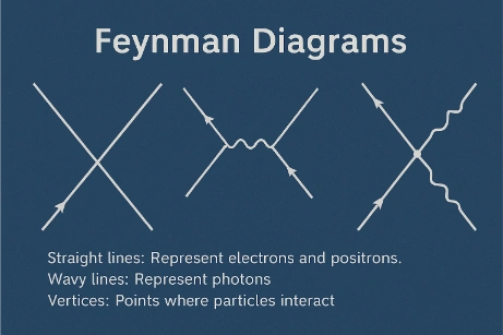
3. What role do Feynman diagrams play in QED?
Answer: Feynman diagrams provide a visual and calculational tool for representing the interactions of particles in QED. They depict the paths of particles and the exchange of virtual photons, simplifying the computation of probability amplitudes for various processes.

4. How does QED describe the interaction between light and matter?
Answer: In QED, light and matter interact through the exchange of virtual photons. This exchange mediates forces between charged particles, allowing QED to accurately predict phenomena such as scattering, pair production, and the Lamb shift.

5. What are virtual particles in the context of QED?
Answer: Virtual particles are transient fluctuations that occur during particle interactions. Although they cannot be directly observed, they are essential in mediating forces in QED, enabling the exchange of energy and momentum between particles.

6. How does QED incorporate the principles of quantum mechanics and special relativity?
Answer: QED merges quantum mechanics with special relativity by treating particles as excitations of underlying fields. It uses relativistic equations and probability amplitudes to describe interactions, ensuring that the theory remains consistent at high energies and speeds.

7. What is the fine-structure constant and why is it important in QED?
Answer: The fine-structure constant, approximately 1/137, is a dimensionless parameter that characterizes the strength of electromagnetic interactions. It plays a crucial role in QED by determining the magnitude of corrections to classical predictions and appears in many QED calculations.

8. What are radiative corrections and renormalization in QED?
Answer: Radiative corrections are adjustments to particle interactions due to the emission and reabsorption of virtual photons. Renormalization is the process of absorbing infinities into redefined parameters, allowing QED to make finite, accurate predictions that match experimental results.

9. What experimental evidence supports the predictions of QED?
Answer: QED is supported by highly precise experimental measurements such as the anomalous magnetic moment of the electron, the Lamb shift in hydrogen, and the outcomes of high-energy particle scattering experiments, all of which match QED predictions to remarkable accuracy.

10. How has QED influenced modern physics and technology?
Answer: QED has profoundly influenced modern physics by providing a framework for understanding electromagnetic interactions with unprecedented precision. Its principles underpin technologies like lasers, semiconductors, and quantum computing, and it has paved the way for further developments in quantum field theory.

QED: Thought-Provoking Questions and Answers:

1. How does QED challenge our classical understanding of electromagnetic interactions?
Answer: QED introduces the concept of quantized fields and virtual particles, which contrast with classical continuous fields. This quantum approach explains phenomena that classical theories cannot, such as spontaneous emission and the discrete energy levels in atoms, reshaping our understanding of nature’s fundamental processes.

2. What are the philosophical implications of virtual particles in QED?
Answer: Virtual particles suggest that the vacuum is not empty but teems with transient fluctuations. This challenges our perception of “nothingness” and has profound implications for our understanding of reality, causality, and the nature of quantum fields.

3. How do Feynman diagrams simplify the calculation of complex quantum processes?
Answer: Feynman diagrams provide a pictorial representation of particle interactions, reducing complex integrals into manageable components. Each diagram corresponds to a mathematical expression, making it easier to visualize and calculate the probability amplitudes of various processes.

4. In what ways does the fine-structure constant influence the behavior of electromagnetic interactions?
Answer: The fine-structure constant determines the strength of electromagnetic interactions. Its small value (~1/137) explains why electromagnetic effects are relatively weak compared to the strong nuclear force, and it governs the magnitude of higher-order corrections in QED calculations.

5. How might future experiments refine our understanding of QED and possibly reveal physics beyond the Standard Model?
Answer: Future high-precision experiments, such as advanced measurements of the electron’s magnetic moment or scattering experiments at higher energies, could expose tiny deviations from QED predictions. Such discrepancies might point to new physics, such as undiscovered particles or forces, and lead to an extended theory beyond the Standard Model.

6. What role does renormalization play in making QED a predictive theory, and what does it imply about the nature of infinities in physics?
Answer: Renormalization systematically removes infinities from QED calculations by redefining parameters like mass and charge. This process not only makes the theory predictive but also suggests that our classical notions of point particles may be approximations, hinting at a deeper underlying structure.

7. How can the principles of QED be applied to emerging technologies like quantum computing and quantum communication?
Answer: QED’s understanding of light–matter interactions and quantum entanglement forms the basis for many quantum technologies. Insights from QED help develop qubits, quantum gates, and secure communication protocols by manipulating and controlling quantum states with high precision.

8. How does the concept of gauge invariance in QED contribute to our understanding of fundamental forces?
Answer: Gauge invariance in QED is the principle that the theory remains unchanged under local transformations of the phase of the wavefunction. This symmetry is fundamental to the conservation of charge and has led to the development of gauge theories that describe all fundamental forces, highlighting the deep connection between symmetry and conservation laws.

9. What challenges remain in unifying QED with the theory of gravity, and how might this impact our understanding of the universe?
Answer: Unifying QED with gravity requires a consistent theory of quantum gravity, which remains one of the biggest challenges in theoretical physics. Overcoming this could lead to a more complete understanding of the universe at both the smallest and largest scales, potentially revealing new insights into black holes, cosmology, and the early universe.

10. How do radiative corrections in QED impact the energy levels of atoms, and what experimental evidence supports these corrections?
Answer: Radiative corrections, such as those leading to the Lamb shift, slightly alter the energy levels of atoms by accounting for interactions with virtual photons. Precision spectroscopy has measured these shifts, confirming the predictions of QED and demonstrating the theory’s accuracy in describing atomic structure.

11. How might advancements in computational techniques and numerical simulations improve our understanding of QED processes?
Answer: Advances in computational methods allow for more precise simulations of QED processes, including complex multi-loop Feynman diagrams. These improvements can lead to better predictions of scattering amplitudes and higher-order corrections, enhancing our understanding of electromagnetic interactions at the quantum level.

12. In what ways does QED provide a framework for exploring the quantum vacuum, and what are the potential implications of this research?
Answer: QED reveals that the quantum vacuum is a dynamic environment filled with fluctuations and virtual particles. Studying these effects can lead to a deeper understanding of phenomena like the Casimir effect, vacuum polarization, and even dark energy, with far-reaching implications for both fundamental physics and cosmology.

QED: Numerical Problems and Solutions:

1. Calculate the Compton wavelength of an electron.
Solution:

Formula:

λC=hmec
h=6.626×1034J/s
me=9.11×1031kg
c=3.00×10⁸m/s
λC=6.626×10349.11×1031×3.00×1082.43×1012m

2. Determine the fine-structure constant α using

α=e24πε0c\alpha = \frac{e^2}{4 \pi \varepsilon_0 \hbar c}

Solution:

e=1.602×10¹⁹C
ε0=8.85×10¹²F/m
=1.055×1034J/s
c=3.00×10⁸m/s
α=(1.602×10¹⁹)24π×8.85×1012×1.055×1034×3.00×1082.566×10381.112×10281/137

3. Compute the energy of a photon with a wavelength of 400 nm.
Solution:  

E=hcλE = \frac{hc}{\lambda}

with

h=6.626×1034J/s

,

λ=400nm=400×109m
E=6.626×1034×3.00×108400×1094.97×1019J E = \frac{6.626 \times 10^{-34} \times 3.00 \times 10^8}{400 \times 10^{-9}} \approx 4.97 \times 10^{-19} \, \text{J}

4. Calculate the rest energy of an electron in MeV.
Solution:  

E0=mec2
me=9.11×1031kg
c=3.00×10⁸m/s
E0=9.11×1031×(3.00×108)28.19×10¹⁴J E_0 = 9.11 \times 10^{-31} \times (3.00 \times 10^8)^2 \approx 8.19 \times 10^{-14} \, \text{J}

  Convert to MeV:

1eV=1.602×10¹⁹J

So,

E08.19×10141.602×1019511,000eV=0.511MeV E_0 \approx \frac{8.19 \times 10^{-14}}{1.602 \times 10^{-19}} \approx 511,000 \, \text{eV} = 0.511 \, \text{MeV}

5. For a photon of energy 2 MeV, find its wavelength.
Solution:  

E=hcλλ=hcE
E=2MeV=2×106×1.602×1019J=3.204×10¹³J λ=6.626×1034×3.00×1083.204×10136.20×1013m \lambda = \frac{6.626 \times 10^{-34} \times 3.00 \times 10^8}{3.204 \times 10^{-13}} \approx 6.20 \times 10^{-13} \, \text{m}

6. Calculate the Bohr magneton,

μB


Solution:  

μB=e2me\mu_B = \frac{e\hbar}{2m_e}


e=1.602×10¹⁹C e = 1.602 \times 10^{-19} \, \text{C}

,

=1.055×1034J/s,  


me=9.11×1031kg m_e = 9.11 \times 10^{-31} \, \text{kg}

. 

μB1.602×1019×1.055×10342×9.11×10319.27×1024J/T \mu_B \approx \frac{1.602 \times 10^{-19} \times 1.055 \times 10^{-34}}{2 \times 9.11 \times 10^{-31}} \approx 9.27 \times 10^{-24} \, \text{J/T}

7. If the electron’s anomalous magnetic moment is 0.00116 times the Bohr magneton, calculate its numerical value in J/T.
Solution:  

Δμ=0.00116×μB0.00116×9.27×1024J/T1.08×1026J/T \Delta\mu = 0.00116 \times \mu_B \approx 0.00116 \times 9.27 \times 10^{-24} \, \text{J/T} \approx 1.08 \times 10^{-26} \, \text{J/T}

8. A scattering experiment measures a QED correction that is 0.1% of the classical value. If the classical cross-section is

1×10281 \times 10^{-28}

m², what is the corrected cross-section?

Solution:
  Corrected cross-section

σ=σclassical×(1+0.001)=1×1028×1.0011.001×1028m2 \sigma = \sigma_{\text{classical}} \times (1 + 0.001) = 1 \times 10^{-28} \times 1.001 \approx 1.001 \times 10^{-28}\, \text{m}^2

9. Calculate the electron cyclotron frequency for a magnetic field of 0.2 T.
Solution:  

ωce=eBme=1.602×1019×0.29.11×10313.52×1010rad/s \omega_{ce} = \frac{eB}{m_e} = \frac{1.602 \times 10^{-19} \times 0.2}{9.11 \times 10^{-31}} \approx 3.52 \times 10^{10} \, \text{rad/s}

10. An electron in a magnetic field of 1.0 T has a cyclotron radius of 0.002 m. Calculate its speed.
Solution:
For circular motion,

r=meveBv=reBme r = \frac{m_e v}{eB} \Rightarrow v = \frac{r eB}{m_e} v=0.002×1.602×1019×1.09.11×10313.204×10229.11×10313.52×108m/s v = \frac{0.002 \times 1.602 \times 10^{-19} \times 1.0}{9.11 \times 10^{-31}} \approx \frac{3.204 \times 10^{-22}}{9.11 \times 10^{-31}} \approx 3.52 \times 10^{8} \, \text{m/s}

11. If a QED process has an amplitude proportional to the fine-structure constant

α

1/137, what is the order of magnitude of the probability (amplitude squared) of this process?
Solution:

Probability ∼α2(1/137)25.33×105 \sim \alpha^2 \approx (1/137)^2 \approx 5.33 \times 10^{-5}

12. The Lamb shift in hydrogen is measured to be about 1057 MHz. Convert this energy shift to joules.
Solution:

Energy E=hν
where h=6.626×1034J/s  and ν=1057×106Hz E6.626×1034×1.057×1097.01×1025J