Prepare for University Studies & Career Advancement
Magnetostatics
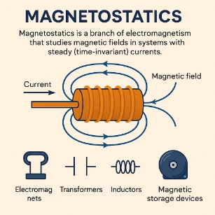
Magnetostatics is the part of physics that studies magnetic fields produced by steady currents and time-independent magnetic systems. It belongs to the wider study of electricity and magnetism, but it focuses on situations where the currents and magnetic fields are not changing with time. This makes magnetostatics a powerful first framework for understanding magnetic fields around wires, loops, coils, solenoids, toroids, permanent magnets, and magnetic materials.
Students often first meet magnetism through simple observations: a compass needle turns, a current-carrying wire affects a nearby magnet, or an electromagnet attracts iron. Magnetostatics gives these observations a deeper structure. It asks how steady electric currents produce magnetic fields, how symmetry helps us calculate those fields, and how materials respond when placed in a magnetic environment.
This hub builds naturally on basic ideas from electrical circuits, where current is introduced as moving charge, and from the wider topic of magnetic fields, where students learn that magnetism has direction, strength, and field-line patterns. It also sits beside electrostatics, which studies static electric fields. Together, electrostatics and magnetostatics prepare students for the more dynamic ideas of electrodynamics, where fields change with time and electromagnetic waves can propagate.
The Magnetostatics cluster is organised around three important learning paths. The Biot–Savart Law shows how magnetic fields can be built from small current elements. Ampère’s Law shows how symmetry and enclosed current can simplify magnetic-field calculations. Magnetic Dipoles and Materials explains how matter responds to magnetic fields through magnetic moments, domains, magnetisation, and material properties.
For university preparation, magnetostatics is valuable because it teaches more than formulas. It trains students to think in terms of fields, geometry, symmetry, vectors, closed paths, material response, and physical modelling. These habits are essential in physics and engineering, especially in topics such as electromagnets, motors, generators, transformers, magnetic sensors, shielding, magnetic materials, and scientific instruments.
The central message is simple: steady currents and magnetic materials shape the magnetic field around them in structured, predictable ways. By learning magnetostatics, students gain a clearer foundation for understanding both classical magnetic phenomena and the more advanced electromagnetic technologies built upon them.
Understanding Magnetostatics: Magnetic Fields from Steady Currents
Steady Magnetic Fields and Material Response
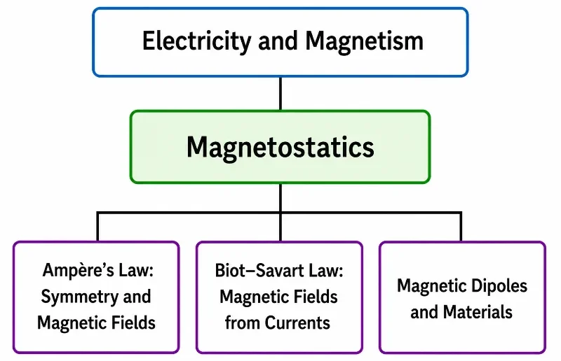
Magnetostatics sits within Electricity and Magnetism and focuses on magnetic fields that arise from steady currents and magnetic materials. This pathway guides students from the wider field of electromagnetism into three connected studies: current-generated fields, symmetry-based field calculation, and the magnetic behaviour of matter.
Provides the wider foundation for electric charge, current, magnetic fields, circuits, induction, waves, and electromagnetic interactions.
Magnetostatics – Overview
Focuses on magnetic fields produced by steady currents and magnetic materials, forming the classical foundation for wires, coils, solenoids, toroids, dipoles, and magnetic media.
Shows how closed paths, enclosed current, and symmetry can simplify magnetic-field calculations for straight wires, solenoids, toroids, and other regular current systems.
Connects magnetic moments, domains, magnetisation, permeability, and material response to real devices such as magnets, sensors, motors, and transformer cores.
Magnetostatics is highlighted as the central hub linking steady-current magnetic fields, symmetry methods, and magnetic materials.
This hierarchy chart shows Magnetostatics as a highlighted sub-cluster within the wider Electricity and Magnetism section. The top node is Electricity and Magnetism, followed by the highlighted Magnetostatics hub. Below it are three related learning pages: Ampère’s Law: Symmetry and Magnetic Fields, Biot–Savart Law: Magnetic Fields from Currents, and Magnetic Dipoles and Materials. The chart helps students see that Magnetostatics connects magnetic-field calculation, current geometry, symmetry, and material response within one coherent learning pathway.
Symmetry Bounds and Ampèrian Line Integrals
To evaluate static magnetic flux distributions mathematically, magnetostatics isolates steady currents where charge density remains constant over time, satisfying the continuity equation identity ∇ · J = 0. This localized conservation rule allows the divergence of the magnetic field vector to vanish identically everywhere, ∇ · B = 0, proving the absolute non-existence of isolated magnetic monopoles across the cosmic horizon. Consequently, the field lines always map out as uninterrupted closed paths. When evaluating systems with high spatial symmetry, taking a line integral around a closed loop translates geometric symmetry metrics directly into enclosed free-current bounds via the differential statement ∇ × B = μ0J. For undergraduate students transitioning to advanced field theory, analyzing these steady boundary states provides a clean mathematical stepping stone before adding the time-dependent displacement current parameters of full electrodynamics.
Mathematical Formulations and Gauge Transformations
To advance beyond basic scalar geometries, university-level analysis requires evaluating the vector magnetic potential, A. Because the magnetic field vector is solenoidal (∇ · B = 0), Helmholtz’s theorem allows the field to be mapped as the curl of a secondary vector field, defined by B = ∇ × A. In static current systems, implementing the Coulomb gauge restriction (∇ · A = 0) simplifies the differential formulation of Ampère’s law down to a vector Poisson equation:
$$\nabla^2 \mathbf{A} = -\mu_0 \mathbf{J}$$
This vector identity fundamentally shifts calculation dynamics. Instead of performing difficult multi-dimensional cross-product integrations via the Biot-Savart equation, fields can be extracted by evaluating independent Cartesian component distributions. This framework is essential when calculating complex boundary transitions where magnetic media interfaces with free space, ensuring that the tangential component of H and the normal component of B maintain strict macro-scale conservation.
Symmetry Profiles: Mapping Common Current Geometries
Calculating magnetic fields in practice requires matching the current distribution to its natural geometric coordinates. The three primary structural setups include:
Infinite Straight Line Currents
Geometric Boundary: Infinite axial line symmetry mapping along a cylinder.Field Behavior: Field lines form concentric, continuous circular vector loops encircling the wire axis. The field magnitude decays inversely with radial distance, following a strict 1/r path scaling.
Infinite Cylindrical Solenoids
Geometric Boundary: Helical surface currents wrapped around a uniform cylinder length.Field Behavior: The exterior magnetic field cancels out completely to zero, while the internal field vectors align as a uniform, homogeneous axial landscape running straight through the center core.
Symmetrical Toroids
Geometric Boundary: A continuous current-carrying coil wrapped into a closed donut profile.Field Behavior: The magnetic field is completely contained within the interior of the donut rings, mapping as circular lines where the flux magnitude varies strictly based on internal radial distance.
The Classical Field Duality
Developing a robust intuition for electromagnetic systems requires evaluating static electricity alongside steady state magnetism. The table below outlines the core structural dualities that govern field physics before time-varying induction parameters are introduced:
Physical Parameter
Electrostatic Field System
Magnetostatic Field System
Primary Source
Stationary Electric Charges (ρ)
Steady Electric Currents (J)
Fundamental Field Vector
Electric Field Intensity (E)
Magnetic Flux Density (B)
Divergence Property
∇ · E = ρ / ε0 (Gauss’s Law)
∇ · B = 0 (No Monopoles)
Curl Property
∇ × E = 0 (Conservative Field)
∇ × B = μ0J (Ampère’s Law)
Potential Model
Scalar Potential (V) where E = -∇V
Vector Potential (A) where B = ∇ × A
Media Parameter
Permittivity of Free Space (ε0)
Permeability of Free Space (μ0)
The Conductor Duality: Dissecting B and H Fields
When analyzing magnetostatics in real matter rather than empty space, field physics splits into two distinct operational vectors:
The Fundamental Flux Density Vector (B)
Physical Definition: Represents the absolute, total microscopic magnetic field acting on moving point charges inside material coordinates.Key Constraint: Always maintains zero net divergence (∇ · B = 0), ensuring its vector lines remain unbroken and continuous across boundary interfaces.
The Auxiliary Magnetic Intensity Vector (H)
Physical Definition: Represents the macroscopic field drive originating exclusively from macro free currents, factoring out atomic bound currents.Key Constraint: Binds directly to free current distributions through the curl line relation (∇ × H = Jfree), serving as the primary diagnostic tool in engineering core circuits.
Magnetostatics — Deep-Dive FAQ Hub
What is magnetostatics?
Magnetostatics is the branch of physics that studies magnetic fields produced by steady (time-independent) electric currents and permanent magnets, where the fields and currents do not change with time. It is the magnetic analogue of electrostatics.
What are the fundamental laws governing magnetostatics?
Magnetostatics relies on laws such as the Biot–Savart law and Ampère’s circuital law, as well as Gauss’s law for magnetism. These laws relate steady currents or permanent magnetisation to the magnetic field they produce.
What does Gauss’s law for magnetism tell us about magnetic field lines?
Gauss’s law for magnetism states that the net magnetic flux through any closed surface is zero, implying that magnetic field lines have no beginning or end and always form closed loops. This reflects the fact that isolated magnetic monopoles do not exist under classical magnetostatics.
How can we compute the magnetic field produced by a steady current?
For steady currents, the Biot-Savart law gives a way to compute the magnetic field at any point by integrating contributions from each infinitesimal segment of current. For symmetric situations (like infinite straight wires or solenoids), Ampère’s loop law can simplify the calculation.
What is the magnetic field around a long straight current-carrying wire?
For a long straight wire carrying a steady current I, the magnetic field at a distance r from the wire forms concentric circles around the wire. Its magnitude decreases with distance and can be derived using Ampère’s law (or Biot-Savart).
What is a solenoid, and how does it generate a nearly uniform magnetic field inside?
A solenoid is a coil of many turns of wire. When a steady current flows through it, the overlapping contributions of each loop lead to a magnetic field inside the coil that is almost uniform and similar to that of a bar magnet. This configuration is widely used in electromagnets, inductors, and magnetic devices.
What is magnetic force between current-carrying conductors in magnetostatics?
In magnetostatics, two parallel current-carrying wires exert a magnetic force on each other: if currents flow in the same direction they attract; if in opposite direction they repel. This force arises because each wire produces a magnetic field (via its current), and the other wire experiences a force from that field.
When does magnetostatics cease to be a valid approximation?
Magnetostatics assumes that currents and fields are time-independent (steady). If currents change rapidly, or if time-varying electric fields become important, then the full set of electromagnetic equations (with displacement current) must be used instead of the static approximation.
Why is magnetostatics useful, despite being an approximation?
Magnetostatics is extremely useful because many practical situations involve steady currents or slowly varying conditions, so that the static approximation holds. It simplifies analysis of magnetic fields, forces, inductance, and device design such as coils, magnets, magnetic circuits, and more.
How does magnetostatics relate to materials and magnetic media?
Magnetostatics can be extended to include magnetized materials (permanent magnets, magnetized media). In such cases, magnetization and bound currents contribute to the overall magnetic field, and material properties like permeability become important. This allows analysis of real magnets, magnetic circuits, and magnetic storage devices.
Industrial Applications: The Practical Mechanics of Static Fields
Steady-state field engineering dictates the operational limits of various industrial, analytical, and energy generation systems. By controlling non-time-varying currents, engineers manipulate spatial flux vectors to establish mechanical force, route flux paths, or capture subatomic parameters:
Heavy-Duty Industrial Electromagnets
The Core Application: Scrap yard sorting cranes, magnetic scrap separators, and heavy high-field lifting fixtures.
The Role of Magnetostatics: By pushing a massive, steady direct current through highly packed winding layers around a ferromagnetic core, engineers maximize the interior magnetic flux density. Magnetostatic field modeling ensures the core stays below its magnetic saturation limit, providing optimal, predictable lifting forces safely.
Medical Diagnostics: Magnetic Resonance Imaging (MRI)
The Core Application: Clinical high-fidelity soft tissue imaging scanners.
The Role of Magnetostatics: MRI machines rely on massive superconducting coils to maintain an intensely strong, perfectly uniform static magnetic field (typically 1.5 T to 3.0 T) inside the scanning bore. This constant field forces the random nuclear spins of hydrogen atoms in the patient’s body to align perfectly along a single vector baseline, creating a baseline state before dynamic RF pulses are introduced.
Electrical Core Circuit Components
The Core Application: Direct current inductors, ballast chokes, and the steady-state bias tuning arrays in transformer systems.
The Role of Magnetostatics: When Direct Current (DC) runs through an inductive coil, it establishes a steady, time-independent energy storage buffer within the magnetic field volume. Magnetostatic boundary equations are used to design custom air gaps in the iron cores, preventing the steady free currents from triggering magnetic saturation and ensuring high inductance remains stable during operation.
Magnetic Deflection Shielding
The Core Application: Protecting sensitive scientific instruments, electron microscopes, and aerospace navigation sensors from stray magnetic interference.
The Role of Magnetostatics: High-permeability alloy shells (such as Mu-Metal) act as high-efficiency bypass routes for external magnetic field lines. Magnetostatic field mapping lets engineers design geometric layers that channel ambient flux lines smoothly around a protected interior cavity, dropping the internal field strength to near-zero without needing an active power source.
Evolution of Magnetostatics: History, Challenges, and Frontiers
To anchor your structural understanding of steady-state magnetic distributions, it is essential to trace how magnetostatics evolved from mechanical observations into an exact field theory, while exploring the engineering limitations and industrial application frameworks defining tomorrow’s frontier systems.
Historical Epochs: From Oersted’s Compass to Maxwell’s Synthesis
The quantitative era of magnetostatics was ignited in the spring of 1820, when Danish physicist Hans Christian Ørsted noticed that an active electric current deflected a nearby compass needle. This was the first empirical proof linking electricity and magnetism. Within months of learning about Ørsted’s discovery, French physicists Jean-Baptiste Biot and Félix Savart formalized the exact differential mechanics detailing how an infinitesimal line element of current projects a fractional magnetic field vector into space. Concurrently, André-Marie Ampère developed his circuital loop integral law, establishing a mathematical framework that derived magnetic field loops directly from enclosed free currents. This classical epoch culminated in the 1860s when James Clerk Maxwell consolidated these separate steady-state equations into his comprehensive electromagnetic vector field equations, anchoring magnetostatics as the time-independent limit of classical electrodynamics.
Contemporary Engineering Challenges: Flux Leakage, Hysteresis, and Thermal Dissipation
While calculating steady-state fields across ideal geometries is structurally straightforward, managing these distributions in practical industrial machinery reveals massive engineering obstacles. Ferromagnetic transformer cores, electric motor stators, and magnetic shielding arrays do not behave like empty space; they possess complex atomic boundary properties. When designing heavy electromagnets, engineers must battle magnetic flux leakage, where field lines slip outside their intended pathways and disrupt nearby circuitry. Furthermore, real magnetic media suffers from non-linear magnetic hysteresis loops—energy lost as heat as domains physically rub and struggle to realign when fields change. This internal molecular friction, combined with the heavy Joule heating (I2R) generated by pushing thousands of amperes of steady current through copper coils, requires intense active liquid-cooling systems and advanced alloy geometries to prevent thermal failure.
Future Technological Horizons: Spin-Transfer Torques, Cloaking Metamaterials, and High-Field Fusion
The modern frontier of magnetostatics is moving beyond bulk macroscopic conductors toward sub-micron quantum systems. Next-generation Spintronic Data Storage architectures bypass moving parts entirely; they utilize localized static spin polarized currents to execute non-volatile Spin-Transfer Torques (STT), flipping individual atomic magnetic domains to multiply global drive densities and processing speeds. Simultaneously, materials scientists are synthesizing artificial engineering constructs called magnetic metamaterials. By tailoring anisotropic spatial permeability configurations, these advanced structures can deliberately route magnetic field lines around sensitive electronic cavities—effectively creating static magnetic cloaking shields. Finally, tomorrow’s carbon-free power grids rely heavily on advancements in high-field magnetostatics, where high-temperature superconducting magnets maintain massive, steady-state magnetic confinement landscapes to trap hyper-hot plasma inside commercial nuclear fusion reactors.
Review Questions and Answers
What is magnetostatics?
Answer: Magnetostatics is the branch of electromagnetism that studies magnetic fields in systems where the currents are steady (time-independent) and the magnetic fields do not change with time.
How is Gauss’s law for magnetism stated, and what does it imply about magnetic monopoles?
Answer: Gauss’s law for magnetism states that the net magnetic flux through any closed surface is zero, implying that magnetic monopoles do not exist and magnetic field lines form closed loops.
What are the primary sources of magnetic fields in magnetostatics?
Answer: The primary sources are steady electric currents (such as those in wires, coils, and solenoids) and permanent magnets, which have intrinsic magnetic moments due to electron spin and orbital motion.
How does the right-hand rule help in determining the direction of the magnetic field around a current-carrying conductor?
Answer: By pointing your thumb in the direction of the conventional current, your curled fingers indicate the circular direction of the magnetic field lines encircling the conductor.
What is the significance of the magnetic dipole moment in magnetostatics?
Answer: The magnetic dipole moment quantifies the strength and orientation of a magnet or current loop. It determines the torque a magnetic dipole experiences in an external magnetic field and is key to understanding magnetic interactions.
How do you calculate the magnetic field produced by a long, straight current-carrying wire?
Answer: The magnetic field at a distance r from a long, straight wire carrying current I is given by:
$$B = \frac{\mu_0 I}{2\pi r}$$
where μ0 is the permeability of free space.
What role do permanent magnets play in magnetostatics?
Answer: Permanent magnets generate a steady magnetic field due to the alignment of magnetic domains within the material, and their fields can interact with currents and other magnets in various applications.
How does the concept of superposition apply to magnetic fields?
Answer: The principle of superposition states that the net magnetic field at any point is the vector sum of the magnetic fields produced by each individual source, allowing complex field configurations to be analyzed by summing simpler fields.
What is the relationship between the magnetic vector potential and the magnetic field?
Answer: The magnetic field is the curl of the magnetic vector potential:
$$\mathbf{B} = \nabla \times \mathbf{A}$$
a concept that simplifies solving for the field in complex geometries and is useful in advanced theoretical treatments.
How are magnetic fields used in practical applications such as MRI and magnetic storage?
Answer: In MRI, strong, uniform magnetic fields align the nuclear spins of atoms in the body, while gradients and radiofrequency pulses provide imaging data. In magnetic storage, data is encoded by altering the magnetic orientation of small regions in a material.
Thought-Provoking Questions and Answers
How does the absence of magnetic monopoles, as implied by Gauss’s law for magnetism, influence our understanding of magnetic field lines?
Answer: Without magnetic monopoles, magnetic field lines always form closed loops, meaning that every field line that exits a magnet’s north pole must eventually enter its south pole. This symmetry shapes our theoretical models and differentiates magnetism fundamentally from electrostatics, where isolated charges can exist.
In what ways can computational modeling enhance the analysis of complex magnetic field distributions in engineered devices?
Answer: Computational modeling, such as finite element analysis, enables precise simulation of magnetic field distributions in complex geometries. It helps optimize device designs, predict performance under varying conditions, and reduce the need for extensive prototyping, ultimately accelerating technological innovation.
How might novel magnetic materials, such as metamaterials, revolutionize the control of static magnetic fields?
Answer: Metamaterials can be engineered to exhibit unconventional magnetic properties, like negative permeability or tailored anisotropy. These properties can be used to focus or redirect magnetic fields in ways that conventional materials cannot, opening up new possibilities for high-efficiency transformers, cloaking devices, and advanced sensors.
How can the principle of superposition be applied to design magnetic shielding in sensitive electronic equipment?
Answer: By understanding that the net magnetic field is the sum of individual fields, engineers can design multi-layered shields that cancel unwanted external magnetic fields. Optimizing the placement and materials of these layers ensures that sensitive components remain unaffected by interference.
What are the challenges in measuring weak magnetic fields in the presence of strong ambient fields, and how can they be overcome?
Answer: Measuring weak magnetic fields requires high sensitivity and noise reduction. Techniques such as using SQUIDs (superconducting quantum interference devices), differential measurements, and advanced filtering algorithms help isolate and accurately measure weak signals amid stronger ambient fields.
How does the orientation of magnetic domains within a material affect its macroscopic magnetic properties?
Answer: The alignment of magnetic domains determines whether a material exhibits strong permanent magnetism or behaves as a soft magnetic material. Understanding and controlling domain orientation through treatments like annealing can tailor materials for specific applications, from data storage to electric motors.
What potential applications might arise from a deeper understanding of the magnetic vector potential in complex systems?
Answer: The magnetic vector potential simplifies calculations in regions with complicated magnetic fields. Advances in its application could lead to improved designs in electromagnetics, such as more efficient antenna systems, novel magnetic sensors, and enhanced computational techniques in quantum electrodynamics.
How do magnetic fields interact with superconductors, and what are the implications for future energy technologies?
Answer: Superconductors expel magnetic fields through the Meissner effect and can carry large currents with zero resistance. These properties are exploited in technologies like MRI magnets and maglev trains, and they hold promise for lossless power transmission and high-field magnets in fusion reactors.
In what ways can the study of magnetostatics inform our understanding of planetary magnetic fields and space weather?
Answer: Planetary magnetic fields, generated by dynamo processes in a planet’s core, are analyzed using magnetostatic principles. Understanding these fields helps predict space weather, protect satellites from solar storms, and even provide insights into the internal structure and evolution of planets.
How might advancements in measurement techniques impact the future study of static magnetic fields in biological systems?
Answer: Improved sensors and imaging techniques can provide detailed maps of magnetic fields in biological tissues, enhancing our understanding of phenomena such as neural activity and magnetoreception in animals. This research could lead to breakthroughs in medical diagnostics and treatments.
Numerical Problems and Solutions
1. A long, straight conductor carries a current of 10 A. Calculate the magnetic field at a distance of 0.05 m from the wire. (Use μ0 = 4π × 10-7 T·m/A)
Solution: Using the infinite line distribution model:
3. A circular loop with a radius of 0.10 m has 30 turns. If it is placed in a uniform magnetic field of 0.3 T, calculate the magnetic flux through the loop.
Solution: Enclosed structural area evaluated per individual turn element:
$$A = \pi (0.10)^2 \approx 0.0314\text{ m}^2$$
Magnetic flux passing through a single loop boundary:
$$\Phi = BA = 0.3 \times 0.0314 = 0.00942\text{ Wb}$$
Total combined structural loop tracking flux calculated for 30 turns:
4. A rectangular loop of dimensions 0.15 m by 0.10 m is placed in a magnetic field of 0.4 T. Calculate the flux through the loop if it is perpendicular to the field.
Solution: Enclosed spatial geometric area calculation:
$$A = 0.15 \times 0.10 = 0.015\text{ m}^2$$
Flux transformation calculation lines:
$$\Phi = BA = 0.4 \times 0.015 = 0.006\text{ Wb}$$
5. A solenoid has 1000 turns and a length of 0.8 m. If it carries a current of 3 A, calculate the magnetic field inside the solenoid.
Solution: Turns per unit length configuration parameter:
$$n = \frac{1000}{0.8} = 1250\text{ turns/m}$$
Now isolate interior field parameter metrics:
$$B = \mu_0 n I = 4\pi \times 10^{-7} \times 1250 \times 3 \approx 4.71 \times 10^{-3}\text{ T}$$
6. A permanent magnet creates a magnetic field of 0.2 T at a distance of 0.05 m. If the field strength follows an inverse cube law with distance, estimate the field at 0.10 m.
Solution: Following an inverse cube tracking matrix relationship:
7. A bar magnet has a magnetic dipole moment of 0.8 A·m². Calculate the magnetic field at a point along the axial line at a distance of 0.2 m from the magnet’s center.
Solution: Magnetic field calculated directly along the axial linear path:
$$B = \frac{\mu_0}{4\pi} \cdot \frac{2m}{r^3}$$
With constant values μ0 / (4π) = 10-7 T·m/A, dipole value m = 0.8 A·m², and range variable r = 0.2 m:
8. A cylindrical conductor of radius 0.02 m carries a current of 6 A uniformly. Calculate the magnetic field at a point 0.01 m from the center (inside the conductor).
Solution: For internal boundaries inside the current carrier system where r < R:
9. Calculate the total free current enclosed within an Ampèrian loop path if the line integral of the magnetic flux density B evaluated around the entire closed boundary equals precisely 2.5 × 10⁻⁶ T·m.
Solution: Apply the integral statement of Ampère’s circuital law:
Answer: The total static electrical current enclosed within the Ampèrian boundary path measures approximately 1.99 A.
10. An ideal toroid ring contains 2000 tightly wound turns of wire wrapped smoothly around a core. If the internal mean radius of the circular track measures exactly 0.15 m and it carries a steady current of 4.0 A, calculate the magnetic flux density B deep inside the core structure.
Solution: Apply the toroid magnetic core distribution equation derived from Ampère’s integrals:
$$B = \frac{\mu_0 NI}{2\pi r}$$
Substitute our given structural system dimensions:
Answer: The ambient magnetic flux density contained safely within the toroid core measures approximately 1.07 × 10⁻² T.
11. A magnetic dipole moment of 1.2 A·m² is aligned with a uniform magnetic field of 0.25 T. Calculate the potential energy of the dipole in the field.
Solution: Scalar potential energy tracking expression:
12. Two identical bar magnets, each with a magnetic dipole moment of 0.5 A·m², are aligned end-to-end along their axial line and separated by 0.1 m. Estimate the magnitude of the magnetic field at the midpoint between them due to one magnet.
where radius coordinate to midpoint is r = 0.05 m (exactly half the 0.1 m path length), given dipole component m = 0.5 A·m², and constant scalar coefficient μ0 / (4π) = 10-7 T·m/A:
(Note: Since these identical magnets lie along a uniform axial trajectory, their individual vector fields add constructively at the absolute midpoint, yielding a double net field of 1.6 × 10⁻³ T).