
Robotics is an interdisciplinary field that integrates mechanics, control theory, artificial intelligence, electronics, and software engineering to design machines capable of sensing, reasoning, and acting within physical environments. Unlike purely digital AI systems, robots operate in the physical world—subject to gravity, friction, dynamic uncertainty, and deterministic real-time constraints. To achieve autonomy, physical platforms must perceive unstructured surroundings, compute state estimators, solve optimal trajectories, and execute closed-loop motor actuations safely and reliably.
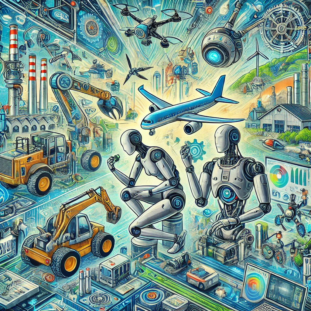
This introductory visualization depicts the convergence of mechanical design, sensor perception, and embedded artificial intelligence. Articulated manipulators, autonomous mobile bases, and distributed feedback sensors operate cohesively under real-time computational architectures, highlighting the multidisciplinary nature of physical automation across research and industrial domains.
This Robotics and Autonomous Systems hub establishes an architectural curriculum spanning the mathematical foundations of articulated mechanics, embodied physical intelligence, distributed middleware, and industrial automation. Each module connects foundational analytical formulations—such as Lie algebra representations of spatial kinematics and nonlinear Lyapunov control—with modern paradigms including Vision-Language-Action (VLA) foundation models, Sim-to-Real policy transfer, and edge tensor acceleration.
The Structure of Robotics Education (IDEF0 Model)
The engineering lifecycle of robotics and autonomous systems education transforms learner curiosity and industrial automation demand into field-ready roboticists and certifiable autonomous deployments. The IDEF0 (Integration Definition for Function Modeling) framework below visualizes the systemic flow of this discipline:
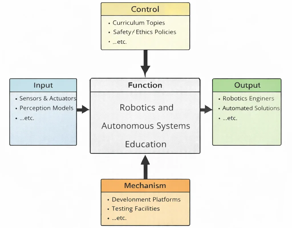
This IDEF0 functional diagram models the core educational transformation process (Node A0). Inputs entering on the left—learner objectives, foundational STEM competencies, and industrial manufacturing constraints—are governed by controls from the top, including ISO safety directives, IEEE robotic standards, and deterministic real-time control constraints. The transformation is executed by operational mechanisms supporting the lower boundary, including ROS 2 middleware stacks, physical testbenches, GPU physics simulators, and sensor fusion suites. The resulting outputs on the right yield certified autonomous roboticists, reproducible open-source software packages, and field-validated physical deployments.
The Sense-Plan-Act Paradigm and Modern Embodied AI
Classical autonomous systems decouple physical operations into the sequential Sense-Plan-Act feedback loop:
- Sensing & State Estimation: Raw streams from exteroceptive sensors (LiDAR point clouds, depth cameras, tactile arrays) and proprioceptive sensors (encoders, IMUs) are fused via Extended Kalman Filters (EKF) or factor graphs to compute real-time pose and obstacle occupancy representations.
- Planning & Decision-Making: Global path planners execute discrete graph searches across topological maps, while local planners compute continuous trajectory optimizations under non-holonomic kinematic constraints, actuator bounds, and collision envelopes.
- Execution & Low-Level Actuation: Trajectory setpoints are tracked by deterministic control loops (such as Computed Torque Control, Model Predictive Control (MPC), and high-gain PID controllers) operating at multi-kilohertz frequencies.
In contemporary Embodied AI, this decoupled pipeline is increasingly unified through end-to-end neural architectures. Vision-Language-Action (VLA) foundation models map continuous multimodal sensory observations directly to joint velocity setpoints, while deep reinforcement learning policies trained inside high-fidelity GPU simulators (such as Isaac Sim) achieve robust Sim-to-Real transfer through aggressive domain randomization.
Mathematical Formulations in Robotics Engineering
Modern robotics relies on rigorous analytical models to represent geometry, kinematics, and dynamics in \(SE(3)\) space:
1. Forward and Inverse Kinematics: A serial manipulator composed of \(n\) joints maps joint coordinates \(\mathbf{q} \in \mathbb{R}^n\) to end-effector pose \(\mathbf{T} \in SE(3)\) via the product of exponentials or Denavit-Hartenberg (D-H) homogeneous transformations:
$$\mathbf{T}_{0}^{n}(\mathbf{q}) = \mathbf{A}_1(q_1) \mathbf{A}_2(q_2) \cdots \mathbf{A}_n(q_n)$$2. Manipulator Differential Kinematics & Jacobians: The geometric Jacobian \(\mathbf{J}(\mathbf{q}) \in \mathbb{R}^{6 \times n}\) maps joint velocity vectors \(\mathbf{\dot{q}}\) to the end-effector spatial twist \(\mathbf{v} = \begin{bmatrix} \boldsymbol{v}^T & \boldsymbol{\omega}^T \end{bmatrix}^T\):
$$\mathbf{v} = \mathbf{J}(\mathbf{q})\mathbf{\dot{q}}$$3. Equations of Motion (Euler-Lagrange Dynamics): The rigid-body dynamic equations governing an articulated robot subject to external wrenches are formulated as:
$$\mathbf{M}(\mathbf{q})\mathbf{\ddot{q}} + \mathbf{C}(\mathbf{q}, \mathbf{\dot{q}})\mathbf{\dot{q}} + \mathbf{g}(\mathbf{q}) = \boldsymbol{\tau} - \mathbf{J}^T(\mathbf{q})\mathbf{f}_{\text{ext}}$$Where \(\mathbf{M}(\mathbf{q})\) is the symmetric positive-definite inertia matrix, \(\mathbf{C}(\mathbf{q}, \mathbf{\dot{q}})\) is the Coriolis and centrifugal matrix, \(\mathbf{g}(\mathbf{q})\) is the gravitational wrench vector, \(\boldsymbol{\tau}\) denotes actuator joint torques, and \(\mathbf{f}_{\text{ext}}\) represents the contact force wrench exerted on the environment.
Foundations of Robot Motion and Mechanics
The mechanical and mathematical backbone of robotics governs physical interaction, dynamic stability, and structural design:
Robot Kinematics and Dynamics: Mathematical modeling of robotic motion, spatial screw theory, coordinate transformations, manipulability ellipsoids, and articulated dynamic equations.
Sensors and Perception in Robotics: Physical sensing modalities, time-of-flight LiDAR, event cameras, and multi-sensor fusion algorithms (Unscented Kalman Filters, Factor Graphs).
SLAM: Localization and Mapping: Algorithms enabling mobile platforms to map unknown topographies while simultaneously estimating position through visual odometry and LiDAR graph SLAM.
Path Planning Algorithms: Algorithmic motion planning across high-dimensional configuration spaces using A*, dynamic window approaches, RRT*, and trajectory optimization schemes (CHOMP, TrajOpt).
Advanced Control Systems in Robotics: State-space feedback, impedance/admittance force control, sliding mode controllers, and nonlinear Model Predictive Control (NMPC).
Actuation and Mechanical Design in Robotics: Brushless permanent magnet motors, harmonic strain-wave gearing, quasi-direct drives, and series elastic actuators (SEAs).
Intelligence and Decision Systems in Robotics
Beyond deterministic kinematics, autonomous robots require adaptive intelligence to reason through high-entropy, dynamic settings:
Evolutionary and Adaptive Robotics: Evolutionary computation and co-design frameworks optimizing both morphology and neural control policies simultaneously.
Reinforcement Learning for Robot Control: Model-free and model-based deep RL, policy gradients (PPO, SAC), and reward shaping applied to legged locomotion and dexterous in-hand manipulation.
Swarm and Multi-Agent Robotics: Decentralized consensus protocols, bio-inspired flocking, and distributed task allocation across multi-robot systems.
Human and Applied Robotics Systems
Applied robotics bridges physical mechanisms with commercial, healthcare, and industrial settings:
Human–Robot Interaction and Ethics: Shared autonomy, ISO 10218/15066 safety standards, intent prediction, and ethical liability frameworks for physical human-robot collaboration.
Industrial Robotics Systems and Cobots: Automated workcells, industrial manipulators, power-and-force-limiting (PFL) collaborative cobots, and high-speed pick-and-place automation.
Medical and Surgical Robotics: Sub-millimeter teleoperated surgical platforms, haptic feedback interfaces, targeted image-guided interventions, and rehabilitation exoskeletons.
Service Robotics: Mobile hospitality platforms, autonomous commercial floor sanitization, and domestic assistive manipulation systems.
Agricultural Robotics: Field phenotyping, autonomous weed removal via targeted vision-laser actuation, and selective robotic harvesting.
Warehouse Logistics and Autonomous Mobile Robots (AMRs): Automated guided vehicles, shelf-lifting AMR fleets, and high-density warehouse dynamic routing.
Aerial Robotics and UAV Systems: Quadrotor aerodynamics, \(\text{SE}(3)\) geometric flight controllers, visual-inertial state estimation, and agile obstacle avoidance.
Autonomous Ground Vehicles: Perception architectures, multi-LiDAR tracking pipelines, behavioural motion planning, and drive-by-wire vehicular platforms.
Robotics Software and Infrastructure
Robust autonomous behavior is underpinned by high-reliability embedded operating systems, deterministic middleware, and distributed computation:
Robot Operating System (ROS and ROS 2): Data Distribution Service (DDS) communication protocols, ROS 2 node lifecycles, and hardware abstraction layer development.
Robotics Simulation Platforms: GPU-accelerated multi-body physics simulators (Gazebo, Isaac Sim, MuJoCo) for mass data generation and policy pre-training.
Real-Time Embedded Systems in Robotics: Microcontroller architectures (ARM Cortex-M/R), Real-Time Operating Systems (FreeRTOS, Zephyr), and deterministic CAN-FD/EtherCAT communication buses.
Robotics Middleware and Distributed Systems: High-throughput, low-latency inter-process communication stacks, zero-copy transport, and edge compute orchestration.
Robotic Digital Twin Systems and Simulation: Closed-loop real-time telemetry streaming, bidirectional synchronization, and predictive degradation monitoring.
Cloud Robotics and Edge Intelligence: Offloaded heavy computing (global SLAM optimization, large model inferencing) to cloud clusters while executing low-latency perception locally.
Soft Robotics and Bio-Inspired Systems: Continuum mechanics, fluidic elastomer actuators, dielectric elastomers, and morphological computation.
Robotics and Quantum Computing: Quantum annealing for large-scale fleet combinatorial routing and quantum algorithms for high-dimensional SLAM optimization.
🎯 Career Guidance Tool Is Robotics & Autonomous Systems Right For You?Explore hardware and software engineering pathways, evaluate your technical fit, and map your trajectory into physical AI. | Explore Career Options → |
- AI – Overview: Core concepts, symbolic reasoning, and modern computational machine learning paradigms.
- Computer Vision: 2D/3D feature extraction, convolutional neural networks, optical flow, and volumetric point cloud processing.
- Natural Language Processing (NLP): Large language models, transformer architectures, and semantic intent comprehension.
- Supervised Learning: Regression, classification, loss optimization, and generalization bounds.
- Unsupervised Learning: Dimensionality reduction, autoencoders, clustering, and density estimation.
- Deep Learning: Multi-layer perceptrons, backpropagation dynamics, and generative models.
- Reinforcement Learning: Markov decision processes, Q-learning, and policy search for closed-loop decision agents.
- Expert Systems: Deterministic inference engines and rule-based knowledge representation.
- Robotics: Embodied intelligence uniting mechanics, perception, planning, and real-time actuation.
End-of-Page Exercises: Review, Thought-Provoking & Engineering Problems
Section 1: Foundational Review Questions & Answers
1. What defines robotics as an interdisciplinary engineering field compared to purely digital AI?
Answer: Robotics integrates physical mechanics, electronics, and control theory with AI software. Unlike disembodied AI algorithms operating exclusively in digital environments, robots must execute computations within real-world physical constraints such as gravity, friction, actuator torque saturation, and deterministic real-time sensor latency.
2. What is the difference between robot kinematics and robot dynamics?
Answer: Kinematics studies the geometric motion of robotic links and joints with respect to time, completely ignoring the forces and torques that induce the motion. Dynamics studies the physical forces, torques, mass moments of inertia, and gravity that cause or result from that motion.
3. What is the fundamental objective of SLAM (Simultaneous Localization and Mapping) in autonomous mobile robots?
Answer: SLAM enables a mobile robot placed within an unknown environment to incrementally construct a consistent geometric map of its surroundings while simultaneously estimating its own exact location within that newly constructed map.
4. How do ROS and ROS 2 (Robot Operating System) facilitate robotic software development?
Answer: ROS and ROS 2 provide an open-source middleware framework featuring hardware abstraction, low-level device drivers, inter-process communication (publish-subscribe topics, services, and actions), package management, and standardized perception and navigation suites.
5. What distinguishes industrial collaborative robots (cobots) from traditional industrial robotic arms?
Answer: Cobots are engineered with integrated joint torque sensors, rounded structural contours, and compliant safety controls (power and force limiting according to ISO/TS 15066) that permit direct, cage-free physical collaboration with human workers.
6. What role do sensor fusion techniques play in autonomous mobile robot perception?
Answer: Sensor fusion algorithms (such as Extended Kalman Filters and graph optimizers) statistically merge asynchronous, noisy data streams from complementary sensors (LiDAR, IMUs, wheel encoders, cameras) into a robust, high-accuracy state estimate that overcomes the failure modes of individual sensors.
7. How does Reinforcement Learning (RL) differ from traditional path planning algorithms?
Answer: Traditional path planners (such as A*, Dijkstra, or RRT*) generate explicit geometric trajectories using deterministic cost maps. Reinforcement learning optimizes behavioral control policies via trial-and-error interactions, mapping high-dimensional observations directly to actions by maximizing cumulative reward signals.
8. What is a robotic digital twin, and how is it applied in manufacturing?
Answer: A robotic digital twin is a high-fidelity virtual simulation model continuously updated via real-time operational telemetry from physical robotic hardware, utilized for offline trajectory programming, cycle-time optimization, and predictive maintenance.
9. What defines Soft Robotics compared to traditional rigid-link mechanisms?
Answer: Soft robotics builds mechanisms from compliant, elastic materials (silicones, hydrogels, flexible polymers) inspired by natural organisms, enabling safe manipulation of fragile objects through distributed physical deformation rather than complex sensor feedback.
10. How do Autonomous Mobile Robots (AMRs) navigate warehouse environments compared to legacy AGVs?
Answer: Automated Guided Vehicles (AGVs) rely on fixed physical infrastructure such as magnetic floor tracks or embedded optical tape. AMRs employ onboard LiDAR, depth vision, and SLAM algorithms to dynamically navigate around unexpected obstacles and compute alternative paths autonomously.
Section 2: Analytical & Thought-Provoking Questions
1. How does the "sim-to-real" gap challenge reinforcement learning deployment in physical robotics?
Answer: Reinforcement learning policies trained in physics simulators often fail upon physical deployment due to unmodeled real-world dynamics, including friction non-linearities, gearbox backlash, sensor latency, and thermal motor changes. Addressing this gap requires domain randomization, system identification, and tactile feedback adaptation.
2. What ethical and safety dilemmas arise when autonomous surgical robots operate with minimal human intervention?
Answer: Autonomous surgical interventions raise legal and ethical questions regarding error liability—distributing responsibility across the supervising surgeon, clinical institution, robot manufacturer, and AI algorithm developer while maintaining patient consent and algorithmic transparency.
3. In multi-agent swarm robotics, how can decentralized local communication prevent catastrophic gridlocks?
Answer: Swarm architectures leverage bio-inspired rules (local repulsion, velocity alignment, and artificial potential field gradients) that allow individual robots to resolve spatial conflicts locally, removing reliance on centralized servers that represent single points of failure.
4. How might quantum computing accelerate trajectory optimization for large autonomous robot fleets?
Answer: Quantum optimization algorithms (such as the Quantum Approximate Optimization Algorithm, QAOA) can solve NP-hard combinatorial multi-agent path finding (MAPF) and fleet routing problems exponentially faster than classical heuristic solvers, enabling real-time optimization of massive warehouse AMR fleets.
5. What cybersecurity vulnerabilities threaten cloud-connected robotic manufacturing lines?
Answer: Cloud-connected robots are susceptible to unauthorized DDS topic injection, man-in-the-middle telemetry tampering, denial-of-service attacks causing safety watchdog trips, and adversarial sensor spoofing that can lead to physical damage.
6. How do ethical frameworks govern human-robot interaction in eldercare and domestic service robotics?
Answer: Social service robotics requires governance concerning privacy (continuous domestic video and audio recording), deceptive emotional attachment, and ensuring autonomous machines assist human dignity without eroding patient autonomy.
7. Why is real-time deterministic computing critical for lower-level robotic motor controllers?
Answer: Standard operating systems introduce non-deterministic thread scheduling jitter. Real-Time Operating Systems (RTOS) guarantee hard task deadline execution for motor feedback loops; timing delays can cause phase lag, high-frequency oscillation, and dynamic instability.
8. What are the environmental and economic trade-offs of deploying autonomous agricultural weed-clearing robots?
Answer: Agricultural robots substantially reduce chemical herbicide runoff, groundwater contamination, and soil compaction through targeted mechanical or laser weeding. However, high initial capital acquisition costs and field charging constraints present economic adoption barriers.
9. How does edge intelligence bridge the latency gap between cloud computing and high-speed aerial drone navigation?
Answer: Edge NPUs and embedded GPUs execute computer vision and obstacle avoidance neural networks locally in under 10 milliseconds, eliminating multi-hundred-millisecond wireless cloud round-trip latencies that would cause high-speed UAV collisions.
10. What philosophical and legal questions arise if an autonomous military UAV executes a lethal strike via machine learning?
Answer: Lethal Autonomous Weapons Systems (LAWS) challenge Geneva Conventions regarding military necessity, distinction, and proportionality, raising the moral question of whether algorithmic systems should ever make life-or-death determinations.
11. How do compliant soft actuators mimic biological muscle systems better than electric servomotors?
Answer: Fluidic and dielectric elastomer soft actuators distribute mechanical deformation continuously across their geometry, offering passive shock absorption and adaptive grasping compliance without requiring stiff mechanical transmissions or active force-torque feedback.
12. How does ROS 2 improve upon original ROS architecture for distributed multi-robot deployments?
Answer: ROS 2 removes the centralized ROS Master single point of failure in favor of the OMG Data Distribution Service (DDS) standard, enabling decentralized discovery, configurable Quality of Service (QoS) profiles for lossy wireless networks, and native TLS/DDS-Security encryption.
Section 3: Numerical Engineering Problems & Solutions
A 2-link planar robotic manipulator has link lengths \(L_1 = 0.5\text{ m}\) and \(L_2 = 0.3\text{ m}\). Calculate the end-effector coordinate position \((x, y)\) when joint angles are \(\theta_1 = 30^\circ\) and \(\theta_2 = 45^\circ\). (Use \(\cos(30^\circ) = 0.866\), \(\sin(30^\circ) = 0.500\), \(\cos(75^\circ) = 0.259\), \(\sin(75^\circ) = 0.966\)).
Planar forward kinematics kinematic mapping: $$x = L_1 \cos(\theta_1) + L_2 \cos(\theta_1 + \theta_2)$$ $$y = L_1 \sin(\theta_1) + L_2 \sin(\theta_1 + \theta_2)$$ Sum of angles: \(\theta_1 + \theta_2 = 30^\circ + 45^\circ = 75^\circ\).
Compute \(x\): $$x = 0.5(0.866) + 0.3(0.259) = 0.433 + 0.0777 = 0.5107\text{ m}$$ Compute \(y\): $$y = 0.5(0.500) + 0.3(0.966) = 0.250 + 0.2898 = 0.5398\text{ m}$$ $$\mathbf{p}_{\text{ee}} = (0.511\text{ m},\ 0.540\text{ m})$$ Final Answer: \((0.511\text{ m},\ 0.540\text{ m})\)
A differential-drive autonomous mobile robot has wheel radius \(r = 0.1\text{ m}\) and track width baseline \(W = 0.5\text{ m}\). If the left wheel rotates at angular speed \(\omega_L = 10\text{ rad/s}\) and the right wheel at \(\omega_R = 15\text{ rad/s}\), calculate the chassis forward linear velocity \(v\) and turning yaw rate \(\omega\).
Individual wheel ground tangential velocities: $$v_L = r \cdot \omega_L = 0.1 \times 10 = 1.0\text{ m/s}$$ $$v_R = r \cdot \omega_R = 0.1 \times 15 = 1.5\text{ m/s}$$ Robot forward linear velocity: $$v = \frac{v_R + v_L}{2} = \frac{1.5 + 1.0}{2} = \frac{2.5}{2} = 1.25\text{ m/s}$$ Robot rotational angular velocity: $$\omega = \frac{v_R - v_L}{W} = \frac{1.5 - 1.0}{0.5} = \frac{0.5}{0.5} = 1.0\text{ rad/s}$$ Final Answer: Linear velocity \(v = 1.25\text{ m/s}\), angular velocity \(\omega = 1.0\text{ rad/s}\).
An autonomous vehicle LiDAR sensor acquires \(300{,}000\) points per second. Each point transmits 3D spatial coordinates \((x, y, z)\) as 32-bit floating-point numbers alongside an 8-bit intensity value. Calculate the uncompressed data rate in Megabits per second (Mbps).
Calculate bits per discrete LiDAR point: $$\text{Bits/point} = (3 \times 32\text{ bits}) + 8\text{ bits} = 96 + 8 = 104\text{ bits}$$ Total bitstream throughput per second: $$\text{Throughput} = 300{,}000\text{ points/s} \times 104\text{ bits/point} = 31{,}200{,}000\text{ bits/s}$$ Convert to Megabits per second (\(1\text{ Mbps} = 10^6\text{ bits/s}\)): $$\text{Data Rate} = \frac{31{,}200{,}000}{10^6} = 31.2\text{ Mbps}$$ Final Answer: \(31.2\text{ Mbps}\)
A robotic joint actuator motor produces a stall torque of \(\tau_{\text{motor}} = 2.0\text{ Nm}\) connected to a gearbox with reduction ratio \(N = 50:1\). Assuming mechanical transmission efficiency \(\eta = 0.85\) (\(85\%\)), calculate the output torque \(\tau_{\text{joint}}\) delivered at the robot joint.
Ideal mechanical gear amplification: $$\tau_{\text{ideal}} = \tau_{\text{motor}} \times N = 2.0\text{ Nm} \times 50 = 100\text{ Nm}$$ Account for mechanical transmission losses: $$\tau_{\text{joint}} = \tau_{\text{ideal}} \times \eta = 100\text{ Nm} \times 0.85 = 85\text{ Nm}$$ Final Answer: Joint output torque is \(85\text{ Nm}\).
An autonomous mobile robot draws an average electrical current of \(I = 5\text{ A}\) from a \(V = 48\text{ V}\) lithium-ion battery pack with total energy capacity \(E = 240\text{ Wh}\). Calculate total capacity in Ampere-hours (Ah) and operational continuous runtime in hours.
Battery charge capacity formulation: $$Q = \frac{E}{V} = \frac{240\text{ Wh}}{48\text{ V}} = 5\text{ Ah}$$ Continuous operational endurance runtime: $$t = \frac{Q}{I} = \frac{5\text{ Ah}}{5\text{ A}} = 1.0\text{ hour}$$ Final Answer: Capacity is \(5\text{ Ah}\); runtime is \(1.0\text{ hour}\).
A perception node publishes camera frames over a ROS 2 DDS network. Over 1,000 transmitted messages, average transport latency is \(\mu = 4.5\text{ ms}\) with standard deviation \(\sigma = 1.2\text{ ms}\). Calculate the upper-bound latency within a \(95\%\) normal confidence interval (\(\mu + 2\sigma\)).
Statistical upper-bound latency formulation: $$\text{Latency}_{\text{upper}} = \mu + 2\sigma$$ Substitute measured values: $$\text{Latency}_{\text{upper}} = 4.5\text{ ms} + 2(1.2\text{ ms}) = 4.5 + 2.4 = 6.9\text{ ms}$$ Final Answer: \(6.9\text{ ms}\)
An industrial assembly robot executes a pick-and-place cycle in \(t_{\text{cycle}} = 2.5\text{ seconds}\). Calculate total parts processed during an uninterrupted 8-hour factory shift.
Convert operational shift time to seconds: $$T = 8\text{ hours} \times 3600\text{ s/hour} = 28{,}800\text{ seconds}$$ Total processed throughput: $$\text{Total Parts} = \frac{T}{t_{\text{cycle}}} = \frac{28{,}800}{2.5} = 11{,}520\text{ parts}$$ Final Answer: \(11{,}520\text{ parts}\)
An AMR uses an Inertial Measurement Unit (IMU) exhibiting an uncalibrated accelerometer bias drift of \(a_{\text{drift}} = 0.02\text{ m/s}^2\). If the AMR travels for \(t = 10\text{ seconds}\) starting from rest without external position correction, calculate the accumulated dead reckoning position error.
Second-order kinematic position integration from constant bias acceleration: $$s_{\text{drift}} = \frac{1}{2} a_{\text{drift}} t^2$$ Substitute parameters: $$s_{\text{drift}} = \frac{1}{2} (0.02\text{ m/s}^2) (10\text{ s})^2 = 0.01 \times 100 = 1.0\text{ meter}$$ Final Answer: Position drift error is \(1.0\text{ meter}\).
An electromagnetic robotic gripper generates an attractive holding force proportional to the square of magnetic flux density: \(F \propto B^2\). If the coil flux density is increased by \(50\%\) (new flux \(B_1 = 1.5 B_0\)), calculate the percentage increase in holding force.
Force scaling ratio: $$\frac{F_1}{F_0} = \left(\frac{B_1}{B_0}\right)^2 = (1.5)^2 = 2.25$$ Percentage increase calculation: $$\Delta F\% = \left(\frac{F_1 - F_0}{F_0}\right) \times 100\% = (2.25 - 1.0) \times 100\% = 125\%$$ Final Answer: Holding force increases by \(125\%\) (delivering \(2.25\times\) the original force).
A logistics facility deploys a fleet of \(N = 20\text{ AMRs}\), each drawing \(P_{\text{charge}} = 3.5\text{ kW}\) when docked at rapid DC fast-charging terminals. If \(40\%\) of the fleet charges concurrently during shift changeover, calculate the total active electrical power demand.
Number of active charging stations: $$N_{\text{active}} = 20 \times 0.40 = 8\text{ robots}$$ Total simultaneous facility power demand: $$P_{\text{total}} = N_{\text{active}} \times P_{\text{charge}} = 8 \times 3.5\text{ kW} = 28.0\text{ kW}$$ Final Answer: Total charging electrical demand is \(28\text{ kW}\).
An RTOS scheduler executes a high-priority motor joint servo control task requiring execution budget \(C = 2\text{ ms}\) repeating on a fixed loop period \(T = 10\text{ ms}\). Calculate the single-task CPU utilization factor \(U\).
Liu and Layland CPU task utilization ratio: $$U = \frac{C}{T}$$ Substitute parameters: $$U = \frac{2\text{ ms}}{10\text{ ms}} = 0.20 \Rightarrow 20\%$$ Final Answer: Task CPU utilization is \(20\%\).
An autonomous ground vehicle cruises at \(v_0 = 20\text{ m/s}\). Upon detecting an obstacle, perception-to-actuation system latency is \(t_{\text{latency}} = 0.2\text{ seconds}\), after which emergency disc brakes deliver constant deceleration \(a = 5\text{ m/s}^2\). Calculate the total distance traversed before coming to a complete stop.
Reaction distance during compute latency: $$d_{\text{react}} = v_0 \times t_{\text{latency}} = 20\text{ m/s} \times 0.2\text{ s} = 4.0\text{ meters}$$ Mechanical braking deceleration distance: $$d_{\text{brake}} = \frac{v_0^2}{2a} = \frac{(20)^2}{2(5)} = \frac{400}{10} = 40.0\text{ meters}$$ Total stopping distance: $$d_{\text{total}} = d_{\text{react}} + d_{\text{brake}} = 4.0 + 40.0 = 44.0\text{ meters}$$ Final Answer: Total stopping distance is \(44.0\text{ meters}\).
Robotics and Autonomous Systems — Summary & Wrap-Up
Robotics and Autonomous Systems unite mechanical engineering, control theory, artificial intelligence, and software infrastructure to build machines capable of intelligent physical action. By mastering forward/inverse kinematics, sensor fusion perception, SLAM mapping, path planning, ROS 2 middleware, and industrial or service deployment, robotics engineers design resilient autonomous systems that transform manufacturing, healthcare, logistics, and planetary exploration.