
Traditional robotic control systems rely heavily on mathematical models derived from physical laws. Engineers describe a robot's motion using differential equations of dynamics, then design feedback controllers that compute the torques or forces needed to track desired trajectories.
Reinforcement Learning (RL) introduces a fundamentally different paradigm. Instead of deriving control strategies analytically, an autonomous robot learns control policies directly through environmental interaction. By repeatedly executing actions and observing the resulting state transitions and rewards, the robot optimizes its decision-making strategies to produce desired behaviors.
Rather than solving control equations symbolically, RL algorithms optimize parameterized policies by maximizing the expected cumulative discounted reward obtained over time.
In physical robotics, this data-driven formulation is especially advantageous when dynamics exhibit:
- Severe non-linearities and unmodeled friction
- Complex hydrodynamic, aerodynamic, or soft-material deformations
- Unpredictable, intermittent physical contact forces (e.g., legged locomotion, multi-fingered grasping)
- Non-stationary operating environments and payload variations
Instead of relying on an explicit analytical model, the robot learns a mapping from observed states to actuator actions through trial and feedback. Control is thereby reframed as a problem of sequential decision-making under uncertainty.
This approach forms a foundational pillar of the Intelligence and Decision Systems in Robotics curriculum, connecting with:
Together, these disciplines investigate how autonomous agents can learn, adapt, and coordinate complex behaviors without requiring exhaustive manual programming.
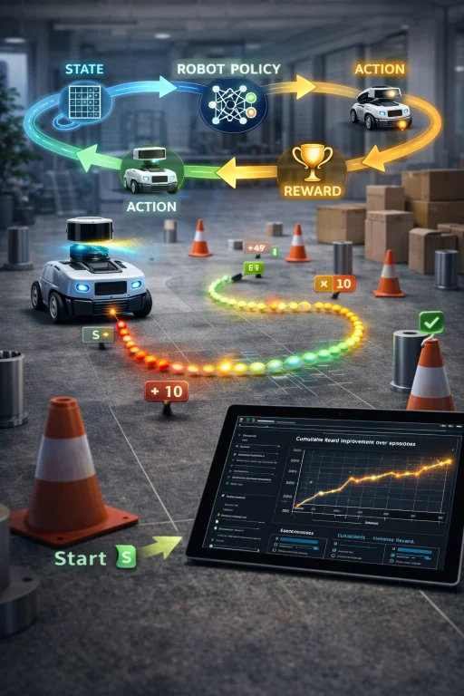
This architecture illustrates an autonomous agent learning closed-loop motor control policies through continuous environmental interaction. The agent observes state vectors (joint angles, velocities, spatial sensor streams), selects action commands via a parameterized policy, and receives immediate scalar rewards. Over extended training horizons, policy gradient and value-based optimization algorithms adjust neural network weights to maximize expected long-term return, resolving control tasks where analytical dynamic modeling is mathematically intractable.
Interactive Quick Review: Fundamentals of Reinforcement Learning
Test your understanding of model-free reinforcement learning versus classical model-based control before exploring Markov Decision Processes:
1. What is the fundamental difference in control strategy discovery between classical control and reinforcement learning?
Answer: Classical control derives control laws analytically using explicit differential dynamic equations (e.g., Newton-Euler, Euler-Lagrange), whereas reinforcement learning discovers control policies empirically through closed-loop trial-and-error environmental interaction to maximize cumulative reward.
2. When is reinforcement learning particularly advantageous over classical mathematical modeling in robotics?
Answer: When system dynamics are highly non-linear, mathematically intractable to derive symbolically, subject to discontinuous contact mechanics (such as bipedal footfalls or multi-finger dexterous grasping), or exposed to unmodeled environmental changes.
Glossary of Key Terminology
Essential mathematical concepts governing stochastic processes, policy optimization, and deep continuous reinforcement learning:
Markov Decision Process Formulation
Reinforcement learning problems in robotics are formally framed as a Markov Decision Process (MDP), specified by the tuple:
$$\mathcal{M} = (\mathcal{S}, \mathcal{A}, \mathcal{P}, \mathcal{R}, \gamma)$$where:
- \(\mathcal{S}\): continuous or discrete set of reachable states (e.g., joint positions \(\mathbf{q}\), velocities \(\dot{\mathbf{q}}\), and end-effector poses)
- \(\mathcal{A}\): continuous or discrete set of executable actions (e.g., motor drive torques \(\boldsymbol{\tau}\) or commanded velocities)
- \(\mathcal{P}(s' \mid s, a) = \mathbb{P}(s_{t+1} = s' \mid s_t = s, a_t = a)\): stochastic state transition probability distribution describing plant and environment dynamics
- \(\mathcal{R}(s, a, s')\): scalar reward function evaluating immediate transition quality
- \(\gamma \in [0, 1)\): temporal discount factor weighting immediate versus long-term returns
The goal is to discover an optimal policy \(\pi^*(a \mid s)\) that maximizes the expected discounted cumulative return \(J(\pi)\):
$$J(\pi) = \mathbb{E}_{\tau \sim \pi} \left[ \sum_{t=0}^{\infty} \gamma^t \mathcal{R}(s_t, a_t) \right]$$where \(\tau = (s_0, a_0, s_1, a_1, \dots)\) denotes the state-action trajectory generated under policy \(\pi\).
Value Functions and Bellman Optimality
Value functions quantify the expected return achievable from a given state or state-action pair under policy \(\pi\).
The State-Value Function \(V^\pi(s)\) is defined as:
$$V^\pi(s) = \mathbb{E}_\pi \left[ \sum_{k=0}^{\infty} \gamma^k \mathcal{R}(s_{t+k}, a_{t+k}) \;\middle|\; s_t = s \right]$$The Action-Value Function \(Q^\pi(s, a)\) evaluates expected return after taking arbitrary action \(a\) in state \(s\):
$$Q^\pi(s, a) = \mathbb{E}_\pi \left[ \sum_{k=0}^{\infty} \gamma^k \mathcal{R}(s_{t+k}, a_{t+k}) \;\middle|\; s_t = s, a_t = a \right]$$The relationship between \(V(s)\) and \(Q(s, a)\) satisfies:
$$V^\pi(s) = \int_{\mathcal{A}} \pi(a \mid s) Q^\pi(s, a) \, da$$At optimality, the action-value function satisfies the non-linear Bellman Optimality Equation:
$$Q^*(s, a) = \mathcal{R}(s, a) + \gamma \int_{\mathcal{S}} \mathcal{P}(s' \mid s, a) \max_{a' \in \mathcal{A}} Q^*(s', a') \, ds'$$This recursive identity forms the foundation of value-iteration, Q-learning, and deep Q-networks (DQN).
Model-Free Temporal Difference (TD) Q-Learning
When transition probabilities \(\mathcal{P}\) are unknown, Q-learning updates action values directly from experience tuples \((s, a, r, s')\):
$$Q(s, a) \leftarrow Q(s, a) + \alpha \left[ r + \gamma \max_{a'} Q(s', a') - Q(s, a) \right]$$where \(\alpha \in (0, 1]\) denotes the learning rate, and the bracketed expression represents the Temporal Difference error \(\delta_{\text{TD}}\):
$$\delta_{\text{TD}} = r + \gamma \max_{a'} Q(s', a') - Q(s, a)$$Continuous Action Spaces & Policy Gradient Methods
Physical robot joints require continuous control signals (such as motor torques or target angles) rather than discrete action bins. Discretizing high-dimensional continuous action spaces causes exponential combinatorial explosion.
Policy gradient methods directly parameterize a continuous control policy \(\pi_\theta(a \mid s)\) with neural network weights \(\theta\). The objective is to maximize expected performance \(J(\theta)\) via gradient ascent:
$$\theta \leftarrow \theta + \eta \nabla_\theta J(\theta)$$By the Policy Gradient Theorem, the analytical gradient is computed without requiring an explicit environmental dynamics model:
$$\nabla_\theta J(\theta) = \mathbb{E}_{\tau \sim \pi_\theta} \left[ \sum_{t=0}^{T} \nabla_\theta \log \pi_\theta(a_t \mid s_t) \, Q^{\pi_\theta}(s_t, a_t) \right]$$In continuous Gaussian policies, actions are sampled from a normal distribution:
$$a_t \sim \mathcal{N}\left( \mu_\theta(s_t), \Sigma_\theta(s_t) \right)$$where the neural network outputs state-dependent mean actions \(\mu_\theta(s)\) and covariance \(\Sigma_\theta(s)\).
Standard Continuous RL Algorithms in Robotics
- Deep Deterministic Policy Gradient (DDPG): An off-policy actor-critic algorithm utilizing deterministic policy gradients \(\nabla_\theta J \approx \mathbb{E}[\nabla_a Q(s, a) \nabla_\theta \pi(s)]\) combined with target networks and experience replay.
- Proximal Policy Optimization (PPO): An on-policy actor-critic framework that stabilizes training by clipping the probability ratio \(r_t(\theta) = \frac{\pi_\theta(a_t \mid s_t)}{\pi_{\theta_{\text{old}}}(a_t \mid s_t)}\) within a trust-region bound \([1-\epsilon, 1+\epsilon]\).
- Soft Actor-Critic (SAC): An off-policy actor-critic method based on maximum-entropy reinforcement learning, optimizing both expected return and action entropy \(\mathcal{H}(\pi)\) to promote robust exploration: $$J(\pi) = \mathbb{E} \left[ \sum_{t=0}^{\infty} \gamma^t \left( \mathcal{R}(s_t, a_t) + \alpha_{\text{ent}} \mathcal{H}(\pi(\cdot \mid s_t)) \right) \right]$$
Engineering Challenges & Technical Solutions
Deploying reinforcement learning on physical robotic mechanisms introduces distinct challenges not present in purely software environments:
The Challenge: Physics simulators (e.g., MuJoCo, Isaac Gym, Bullet) use simplified contact mechanics, rigid-body approximations, and zero-latency models. Policies optimized purely in simulation frequently fail or exhibit violent oscillations when transferred to real hardware due to unmodeled joint backlash, cable stretch, and thermal motor changes.
- Domain Randomization: Uniformly or normally varying simulated friction, link masses, center-of-mass positions, and latency parameters during training to force the policy to learn robust behaviors.
- System Identification & Real2Sim: Using hardware sensor logs to calibrate simulation parameters (such as motor damping coefficients) before deploying policies.
The Challenge: Model-free RL requires trial-and-error exploration. Unconstrained exploration on a physical robot can command destructive joint torques, slam mechanisms into hard mechanical stops, strip gearboxes, or endanger nearby operators.
- Control Barrier Functions (CBFs): Enforcing mathematical invariance filters that project raw neural network actions \(\boldsymbol{\tau}_{\text{RL}}\) onto the nearest safe, admissible set satisfying joint velocity, acceleration, and contact limits.
- Residual Reinforcement Learning: Layering an RL agent on top of a baseline classical controller (\(\boldsymbol{\tau} = \boldsymbol{\tau}_{\text{classical}} + \pi_\theta(s)\)), ensuring that nominal tracking and basic physical stability are preserved throughout training.
The Challenge: Model-free continuous algorithms typically require millions of interaction steps to converge. Conducting these trials directly on real hardware is physically impractical due to component wear and long test durations.
- Massively Parallel GPU Physics Engines: Simulating tens of thousands of robot instances concurrently in GPU memory (e.g., NVIDIA Isaac Gym), compressing weeks of training time into minutes.
- Off-Policy Experience Replay: Utilizing large replay buffers that allow algorithms (such as SAC or TD3) to reuse past transition tuples repeatedly across training updates.
The Challenge: High-bandwidth robot joint controllers operate at 500 Hz to 1 kHz (\(T_s = 1\text{–}2\text{ ms}\)). Executing forward inference passes on deep multi-layer neural networks on embedded microcontrollers can exceed these deadlines, causing control instability.
- TensorRT & INT8 Quantization: Compiling trained policy networks into quantized fixed-point inference engines optimized for onboard embedded edge GPUs or NPUs.
- Hierarchical Control Architectures: Running the deep RL policy at a lower frequency (e.g., 20–50 Hz) to output position/velocity setpoints, which are tracked by an embedded microcontroller running a deterministic PID loop at 1 kHz, as detailed in Real-Time Embedded Systems in Robotics.
Interactive Quick Review: Bellman Equations, Policy Gradients & Sim-to-Real
Reinforce key concepts regarding Bellman updates, continuous torque control, and domain randomization before reviewing the FAQ:
1. How does the Bellman optimality equation evaluate the value of an action \(Q^*(s, a)\)?
Answer: By summing the immediate observed reward \(\mathcal{R}(s, a)\) with the discounted expected optimal return of the next state: \(\gamma \sum_{s'} \mathcal{P}(s' \mid s, a) \max_{a'} Q^*(s', a')\).
2. What role does domain randomization play in bridging the sim-to-real gap (\(\pi_{\text{real}} \approx \pi_{\text{sim}}\))?
Answer: Domain randomization introduces controlled variations into simulation parameters (such as surface friction, link inertia, sensor noise, and actuator delay), teaching the policy to remain stable across a broad range of real-world dynamic conditions.
External References and Further Reading
To explore foundational literature, research algorithms, and benchmark environments in robotic reinforcement learning, consult these resources:
- Reinforcement Learning: An Introduction (Sutton & Barto) – The foundational textbook covering Markov Decision Processes, value function approximation, Q-learning, and policy gradient theory.
- OpenAI Spinning Up in Deep RL – An educational resource providing detailed mathematical derivations and reference implementations for DDPG, PPO, and SAC algorithms.
- IEEE Transactions on Robotics (T-RO) – Peer-reviewed academic journal publishing research on deep reinforcement learning, safe exploration, and sim-to-real transfer for robotic manipulators and legged robots.
Frequently Asked Questions about Reinforcement Learning for Robot Control
What is the difference between model-free and model-based reinforcement learning in robotics?
Model-free RL (e.g., PPO, SAC) maps observations directly to actions through environmental experience without building an explicit mathematical model of the robot or environment. Model-based RL explicitly learns or uses a transition dynamics model \(\mathcal{P}(s' \mid s, a)\) to forecast future states and plan actions via trajectory optimization.
Why is reward shaping critical and challenging in continuous robot control?
Reward functions mathematically define system objectives (e.g., \(\mathcal{R} = -\|\mathbf{q} - \mathbf{q}_d\|^2 - \lambda \|\boldsymbol{\tau}\|^2\)). If weights are misaligned, robots can exploit reward loopholes—discovering erratic, high-frequency motions that score well numerically while causing severe mechanical wear or hardware damage.
How do actor-critic architectures handle continuous motor torques?
Actor-critic methods separate control into two networks: the Actor outputs continuous motor commands (such as joint torques \(\boldsymbol{\tau} = \pi_\theta(s)\)), while the Critic estimates the value function \(Q^\pi(s, a)\) to evaluate action quality and provide gradient updates for the Actor.
What is the "sim-to-real gap," and why does it cause real physical robots to fail?
The sim-to-real gap refers to discrepancies between simulated physics models and real-world environments. Unmodeled motor backlash, cable elasticity, micro-friction variations, and sensor latency cause policies optimized in pure simulation to perform erratically or become unstable on real hardware.
End-of-Page Exercises: Review, Thought-Provoking & Engineering Problems
Section 1: Foundational Review Questions & Answers
1. What five mathematical components define a Markov Decision Process tuple \(\mathcal{M}\)?
Answer: The tuple \(\mathcal{M} = (\mathcal{S}, \mathcal{A}, \mathcal{P}, \mathcal{R}, \gamma)\), representing state space \(\mathcal{S}\), action space \(\mathcal{A}\), state transition probability distribution \(\mathcal{P}\), reward function \(\mathcal{R}\), and discount factor \(\gamma\).
2. What is the fundamental recursive equation for optimal action-value functions \(Q^*(s, a)\)?
Answer: The Bellman optimality equation: \(Q^*(s, a) = \mathcal{R}(s, a) + \gamma \sum_{s'} \mathcal{P}(s' \mid s, a) \max_{a'} Q^*(s', a')\).
3. Write the standard model-free temporal difference update rule for Q-learning.
Answer: \(Q(s, a) \leftarrow Q(s, a) + \alpha \left[ r + \gamma \max_{a'} Q(s', a') - Q(s, a) \right]\).
4. How do policy gradient methods update the policy parameter vector \(\theta\)?
Answer: Via gradient ascent on performance return \(J(\theta)\): \(\theta \leftarrow \theta + \eta \nabla_\theta J(\theta)\), where \(\nabla_\theta J(\theta) = \mathbb{E}[\nabla_\theta \log \pi_\theta(a \mid s) Q^{\pi}(s, a)]\).
5. In continuous robot manipulator control, what physical quantities typically comprise state vector \(s\) and action vector \(a\)?
Answer: State vector \(s = [\mathbf{q}, \dot{\mathbf{q}}]^T\) (joint positions and velocities), while output action vector \(a\) represents motor joint torque vector \(\boldsymbol{\tau} = \pi_\theta(s)\).
6. What dual objectives are encouraged by trajectory reward function \(\mathcal{R} = -\|\mathbf{q} - \mathbf{q}_d\|^2 - \lambda \|\boldsymbol{\tau}\|^2\)?
Answer: Minimizing tracking error position displacement (accurate tracking) while penalizing excessive torque commands (energy efficiency and actuator protection).
7. What technique randomly varies simulation physical parameters during training to reduce transfer error?
Answer: Domain randomization.
8. Under an \(\epsilon\)-greedy action selection strategy, what is the probability of selecting an exploratory action?
Answer: Probability \(\epsilon\), while the greedy action is selected with probability \(1 - \epsilon\).
9. How is total sample interaction count calculated across \(N\) training episodes of duration \(T\) time steps?
Answer: Total interaction steps \(= N \times T\).
10. Name three widely used deep reinforcement learning algorithms for continuous robotic torque control.
Answer: Deep Deterministic Policy Gradient (DDPG), Proximal Policy Optimization (PPO), and Soft Actor-Critic (SAC).
Section 2: Analytical & Thought-Provoking Questions
1. How does the Markov property break down in real-world partially observable robotic environments?
Answer: The Markov property assumes the current state observation \(s_t\) contains all information necessary to forecast \(s_{t+1}\). In real robots, sensor occlusions, unmeasured joint compliance, and internal thermal states mean single observations are incomplete. This converts the system into a Partially Observable MDP (POMDP), requiring recurrent architectures (RNNs/LSTMs) or frame history stacking to maintain state context.
2. Why can unconstrained random exploration lead to mechanical failure when deployed on physical quadrupeds?
Answer: Purely exploratory policies sample random motor torques without physical awareness. Commanding sudden opposing torques across joint linkages can strip gearboxes, trigger motor driver over-current faults, or cause severe structural falls. Safe RL frameworks must enforce barrier functions or classical safety filters to intercept hazardous actions.
3. How does off-policy learning (e.g., SAC) improve sample efficiency compared to on-policy learning (e.g., PPO)?
Answer: On-policy methods must discard training rollouts after each policy update step, collecting fresh samples for every iteration. Off-policy algorithms store historical transitions \((s, a, r, s')\) in a Replay Buffer, allowing neural networks to sample and reuse past experiences across thousands of training batches, reducing required real-world samples.
4. Why is entropy maximization explicitly added to the objective function in Soft Actor-Critic (SAC)?
Answer: SAC optimizes return plus policy entropy (\(J(\pi) = \mathbb{E}[\sum R + \alpha \mathcal{H}(\pi)]\)). Maximizing action entropy prevents policies from prematurely converging to narrow, fragile local optima. This encourages multimodal exploration and yields policies that adapt better to unexpected physical perturbations.
5. What causes the credit assignment problem in long-horizon robotic tasks with sparse rewards?
Answer: When an agent receives feedback only upon final task completion (e.g., a single \(+1\) reward after 10,000 steps), the algorithm struggles to determine which intermediate actions were beneficial and which were suboptimal. Overcoming this requires temporal-difference bootstrapping, reward shaping, or curiosity-driven exploration bonuses.
6. How do asymmetric actor-critic architectures accelerate training during simulation?
Answer: During simulation training, the Critic network is provided privileged ground-truth state information (e.g., exact contact forces, friction coefficients, unoccluded obstacle poses). The Actor network receives only noisy, onboard sensor inputs. Once trained, the privileged Critic is discarded, leaving a deployable Actor that operates solely on real-world sensor streams.
7. Why does pure policy gradient optimization suffer from catastrophic policy collapse, and how does PPO prevent it?
Answer: Large gradient updates can shift network weights into parameter regions where the policy performance drops sharply, preventing the agent from collecting useful exploratory data to recover. PPO enforces a clipped surrogate objective that limits probability updates to a narrow trust region \([1-\epsilon, 1+\epsilon]\), ensuring stable learning steps.
8. How does residual reinforcement learning combine classical control with deep RL?
Answer: Residual RL sets motor torque as the sum of a baseline classical controller and a learned neural network policy (\(\boldsymbol{\tau} = \boldsymbol{\tau}_{\text{classical}} + \pi_\theta(s)\)). The classical controller maintains basic physical stability, while the RL agent learns small residual corrections to compensate for unmodeled friction and complex contact dynamics.
9. What validation challenges emerge when deploying non-deterministic RL policies on safety-critical autonomous systems?
Answer: Deep neural network policies operate as complex non-linear approximations, making formal verification and deterministic failure mode analysis difficult. If an autonomous system encounters out-of-distribution sensor inputs, verifying worst-case bounds requires formal verification tools or deterministic supervisory overrides.
10. How does curriculum learning improve training convergence for dynamic locomotion?
Answer: Attempting to learn dynamic bipedal running directly on rough terrain rarely converges because random exploration fails to find stable gait patterns. Curriculum learning structures training into progressive stages: first maintaining balance, then walking on flat planes, and finally navigating irregular terrain, steadily increasing task difficulty.
11. Why do 1 kHz motor control loops challenge deep RL neural network inference?
Answer: A 1 kHz control loop requires control commands within a 1 millisecond execution window. Forward inference across deep neural networks on embedded microcontrollers can exceed this limit. Systems resolve this via network quantization, TensorRT acceleration, or hierarchical architectures running high-level RL planning at 50 Hz and low-level PID control at 1 kHz.
12. How does state space representation affect sample complexity in robotic manipulation?
Answer: Learning policies directly from raw pixel images requires convolutional layers to simultaneously learn visual representations and motor control laws, requiring millions of interactions. Pre-extracting low-dimensional spatial keypoint vectors (\(s = [x, y, z]^T\)) simplifies the state space, accelerating policy convergence.
Section 3: Numerical Engineering Problems & Solutions
A mobile warehouse robot uses Q-learning to navigate a facility. At state \(s\), executing action \(a\) yields an immediate reward \(r = 3.5\). The robot transitions to next state \(s'\), where the maximum estimated future action-value is \(\max_{a'} Q(s', a') = 12.0\). Prior to the action, the current Q-value estimate was \(Q(s, a) = 7.0\). Given discount factor \(\gamma = 0.85\) and learning rate \(\alpha = 0.20\), calculate the Temporal Difference (TD) target, the TD error signal, and the new updated Q-value \(Q_{\text{new}}(s, a)\).
1. Calculate Temporal Difference target: $$\text{Target} = r + \gamma \max_{a'} Q(s', a') = 3.5 + (0.85 \times 12.0) = 3.5 + 10.2 = 13.7$$ 2. Calculate TD error signal: $$\delta_{\text{TD}} = \text{Target} - Q(s, a) = 13.7 - 7.0 = 6.7$$ 3. Update the Q-value: $$Q_{\text{new}}(s, a) = Q(s, a) + \alpha \delta_{\text{TD}} = 7.0 + (0.20 \times 6.7) = 7.0 + 1.34 = 8.34$$ Final Answer: TD target is \(13.7\), TD error is \(6.7\), and the updated value is \(Q_{\text{new}}(s, a) = 8.34\).
A deep reinforcement learning framework trains a 7-DOF robotic arm policy across \(N = 80,000\) training episodes. Each episode executes for \(T = 250\) control steps. Calculate the total cumulative state-action interaction samples generated during training, and determine the compute time in hours if an accelerated GPU simulator processes steps at a speed of 5,000 interactions per second.
1. Calculate total interaction steps: $$N_{\text{total}} = N \times T = 80,000\text{ episodes} \times 250\text{ steps/episode} = 20,000,000\text{ samples}$$ 2. Compute total time in seconds: $$t_{\text{seconds}} = \frac{20,000,000\text{ steps}}{5,000\text{ steps/s}} = 4,000\text{ seconds}$$ 3. Convert compute time to hours: $$t_{\text{hours}} = \frac{4,000\text{ s}}{3,600\text{ s/hour}} \approx 1.111\text{ hours}$$ Final Answer: Total interaction count is \(20,000,000\text{ samples}\), taking \(1.11\text{ hours}\) of GPU simulation time.
A continuous joint controller evaluates a tracking reward function given by \(\mathcal{R} = -\|\mathbf{q} - \mathbf{q}_d\|^2 - \lambda \|\boldsymbol{\tau}\|^2\). At a specific time step, the joint tracking error vector is \((\mathbf{q} - \mathbf{q}_d) = [0.03, -0.04]^T\text{ radians}\), and the commanded joint torque vector is \(\boldsymbol{\tau} = [2.0, 1.5]^T\text{ N}\cdot\text{m}\). If the energy penalty weighting factor is set to \(\lambda = 0.05\), calculate the squared norms and the exact scalar reward \(\mathcal{R}\).
1. Squared norm of position tracking error: $$\|\mathbf{q} - \mathbf{q}_d\|^2 = (0.03)^2 + (-0.04)^2 = 0.0009 + 0.0016 = 0.0025\text{ rad}^2$$ 2. Squared norm of actuator torque command: $$\|\boldsymbol{\tau}\|^2 = (2.0)^2 + (1.5)^2 = 4.0 + 2.25 = 6.25\ (\text{N}\cdot\text{m})^2$$ 3. Compute scalar reward: $$\mathcal{R} = -0.0025 - (0.05 \times 6.25) = -0.0025 - 0.3125 = -0.3150$$ Final Answer: Evaluated step scalar reward is \(\mathcal{R} = -0.315\).
A policy network parameter weight \(\theta_i\) currently has a value of \(\theta_{\text{old}} = 1.45\). The calculated expected performance return gradient with respect to \(\theta_i\) is evaluated as \(\nabla_\theta J = 3.20\). Using a learning rate step size of \(\eta = 0.05\), calculate the updated policy parameter value \(\theta_{\text{new}}\) following the gradient ascent rule \(\theta \leftarrow \theta + \eta \nabla_\theta J\).
1. Calculate parameter increment: $$\Delta \theta = \eta \nabla_\theta J = 0.05 \times 3.20 = 0.16$$ 2. Apply parameter update: $$\theta_{\text{new}} = \theta_{\text{old}} + \Delta \theta = 1.45 + 0.16 = 1.61$$ Final Answer: Updated policy parameter weight is \(\theta_{\text{new}} = 1.61\).
A discrete Q-learning agent navigates an environment with \(|\mathcal{A}| = 5\) candidate actions. The policy follows an \(\epsilon\)-greedy exploration rule with \(\epsilon = 0.20\) (20% random exploration). Calculate the exact probability assigned to the optimal greedy action \(a^* = \arg\max_a Q(s, a)\), and the probability assigned to each non-greedy exploratory action.
1. Uniform random probability allocated per action: $$P_{\text{rand}} = \frac{\epsilon}{|\mathcal{A}|} = \frac{0.20}{5} = 0.04 \quad (4\%)$$ 2. Probability assigned to each non-greedy action: $$P(a_{\text{non-greedy}}) = P_{\text{rand}} = 0.04 \quad (4\%)$$ 3. Probability assigned to the greedy action \(a^*\): $$P(a^*) = (1 - \epsilon) + P_{\text{rand}} = (1 - 0.20) + 0.04 = 0.80 + 0.04 = 0.84 \quad (84\%)$$ Final Answer: The greedy action probability is \(0.84\ (84\%)\), while each non-greedy action has a probability of \(0.04\ (4\%)\).
A stationary robot policy receives a constant positive step reward \(\mathcal{R}(s_t, a_t) = 4.0\) at every time step over an infinite time horizon. If the system discount factor is set to \(\gamma = 0.90\), use the geometric series formula \(\sum_{t=0}^{\infty} \gamma^t \mathcal{R} = \frac{\mathcal{R}}{1 - \gamma}\) to calculate the exact cumulative discounted return \(G_0\).
1. Apply the infinite geometric sum formula: $$G_0 = \sum_{t=0}^{\infty} \gamma^t \mathcal{R} = \frac{\mathcal{R}}{1 - \gamma}$$ 2. Substitute numerical values: $$G_0 = \frac{4.0}{1 - 0.90} = \frac{4.0}{0.10} = 40.0$$ Final Answer: Total discounted cumulative return sum is \(G_0 = 40.0\).
For a stochastic robot transition model, taking action \(a\) in state \(s\) yields an immediate reward \(\mathcal{R}(s, a) = 1.0\). The robot transitions to state \(s_1'\) with probability \(\mathcal{P}(s_1' \mid s, a) = 0.70\) (where \(V(s_1') = 10.0\)) and to state \(s_2'\) with probability \(\mathcal{P}(s_2' \mid s, a) = 0.30\) (where \(V(s_2') = 5.0\)). Given discount factor \(\gamma = 0.90\), calculate the expected next-state value \(\mathbb{E}[V(s')]\) and determine the total expected action-value \(Q^\pi(s, a)\).
1. Calculate expected next-state value: $$\mathbb{E}[V(s')] = \sum_{s'} \mathcal{P}(s' \mid s, a) V(s') = (0.70 \times 10.0) + (0.30 \times 5.0) = 7.0 + 1.5 = 8.5$$ 2. Apply the Bellman expectation equation: $$Q^\pi(s, a) = \mathcal{R}(s, a) + \gamma \mathbb{E}[V(s')] = 1.0 + (0.90 \times 8.5) = 1.0 + 7.65 = 8.65$$ Final Answer: Expected next-state value is \(8.5\), yielding an action-value of \(Q^\pi(s, a) = 8.65\).
To bridge the sim-to-real gap, an engineer applies domain randomization to a simulated quadruped foot contact friction coefficient \(\mu\). The nominal friction coefficient is \(\mu_{\text{nominal}} = 0.40\). The physics engine randomizes friction uniformly within a \(\pm 30\%\) interval during training. Calculate the minimum friction bound \(\mu_{\text{min}}\) and maximum friction bound \(\mu_{\text{max}}\).
1. Calculate 30% variation margin: $$\Delta \mu = 0.30 \times \mu_{\text{nominal}} = 0.30 \times 0.40 = 0.12$$ 2. Determine lower bound: $$\mu_{\text{min}} = 0.40 - 0.12 = 0.28$$ 3. Determine upper bound: $$\mu_{\text{max}} = 0.40 + 0.12 = 0.52$$ Final Answer: Randomized friction range is \(\mu \in [0.28, 0.52]\).
A Deep Q-Network (DQN) experiences an initial mean squared TD error loss of \(L_1 = 16.0\) during early training iterations. After 50,000 gradient updates, loss drops to \(L_{50\text{k}} = 0.64\). Calculate the absolute loss reduction and the percentage decrease in TD error loss.
1. Absolute loss reduction: $$\Delta L = L_1 - L_{50\text{k}} = 16.0 - 0.64 = 15.36$$ 2. Percentage decrease: $$\% \text{ Reduction} = \frac{\Delta L}{L_1} \times 100 = \frac{15.36}{16.0} \times 100 = 0.96 \times 100 = 96.0\%$$ Final Answer: Absolute loss reduction is \(15.36\), representing a \(96.0\%\) decrease in TD error loss.
An embedded motor controller executes an RL policy network at a control loop sampling rate of \(f_s = 500\text{ Hz}\) (\(T_s = 2.0\text{ ms}\)). Onboard edge-processor benchmarks show sensory feature extraction takes \(t_{\text{vision}} = 0.85\text{ ms}\) and neural network inference takes \(t_{\text{inference}} = 0.95\text{ ms}\). Calculate total processing latency \(T_{\text{exec}}\) and verify whether the real-time deadline \(T_{\text{exec}} \le T_s\) is satisfied.
1. Calculate total execution latency: $$T_{\text{exec}} = t_{\text{vision}} + t_{\text{inference}} = 0.85\text{ ms} + 0.95\text{ ms} = 1.80\text{ ms}$$ 2. Verify against sampling period: $$1.80\text{ ms} \le 2.0\text{ ms} \Rightarrow \text{Condition satisfied}$$ 3. Determine timing margin: $$\text{Margin} = T_s - T_{\text{exec}} = 2.0\text{ ms} - 1.80\text{ ms} = 0.20\text{ ms} \quad (200\ \mu\text{s})$$ Final Answer: Total execution time is \(1.80\text{ ms}\); the system satisfies real-time execution with a \(0.20\text{ ms}\) timing margin.
An \(\epsilon\)-greedy exploration rate decays exponentially across training episodes according to \(\epsilon(k) = \epsilon_0 e^{-\lambda k}\). The initial exploration rate is \(\epsilon_0 = 1.0\), and the decay constant is \(\lambda = 0.0005\text{ episode}^{-1}\). Calculate the exploration rate \(\epsilon\) at episode \(k = 2,000\) (using \(e^{-1.0} \approx 0.36788\)).
1. Calculate the exponent: $$-\lambda k = -0.0005 \times 2,000 = -1.0$$ 2. Evaluate decayed exploration rate: $$\epsilon(2000) = 1.0 \times e^{-1.0} \approx 0.36788 \approx 0.368$$ Final Answer: The exploration rate at episode 2,000 is \(\epsilon \approx 0.368\ (36.8\%)\).
An off-policy continuous RL agent stores transition tuples \((s, a, r, s')\) in a RAM Replay Buffer. State vector \(s\) occupies 64 single-precision floats, action vector \(a\) occupies 8 floats, reward \(r\) occupies 1 float, and next-state \(s'\) occupies 64 floats (total 137 floats per tuple, where 1 float \(= 4\text{ bytes}\)). If replay buffer capacity is set to \(M = 1,000,000\) transitions, calculate the required memory capacity in Megabytes (MB, where \(1\text{ MB} = 10^6\text{ bytes}\)).
1. Bytes required per transition tuple: $$\text{Size}_{\text{tuple}} = 137\text{ floats} \times 4\text{ bytes/float} = 548\text{ bytes}$$ 2. Total byte capacity for 1,000,000 tuples: $$\text{Size}_{\text{total}} = 1,000,000 \times 548\text{ bytes} = 548,000,000\text{ bytes}$$ 3. Convert to Megabytes: $$\text{Memory}_{\text{MB}} = \frac{548,000,000\text{ bytes}}{10^6\text{ bytes/MB}} = 548.0\text{ MB}$$ Final Answer: The replay buffer requires \(548.0\text{ MB}\) of embedded RAM.
Reinforcement Learning for Robot Control — Summary & Wrap-Up
Reinforcement learning reframes robotic control as sequential decision-making under uncertainty, replacing symbolic analytical equations with trial-and-error policy optimization. By mastering Markov Decision Processes, Bellman optimality, Q-learning, policy gradients, continuous actor-critic architectures (DDPG, PPO, SAC), and domain-randomized sim-to-real transfer, engineers build adaptive, resilient autonomous systems capable of discovering optimal control strategies in complex, non-linear environments.
Intelligence and Decision Systems Across the Robotics Ecosystem
Reinforcement learning forms a core pillar of autonomous decision-making, enabling physical machines to acquire complex behavioral skills directly through environmental trial and feedback. These learning paradigms represent a central component of the broader intelligence and decision systems that govern modern autonomous platforms.
Policy search and optimization methods connect closely with techniques studied in Evolutionary and Adaptive Robotics, where population-based search and online adaptation handle environmental uncertainty. Similarly, multi-agent reinforcement learning principles extend directly to Swarm and Multi-Agent Robotics, allowing fleets of autonomous agents to discover decentralized coordination strategies.
Executing complex learned policies on physical hardware relies heavily on underlying computational infrastructure. High-dimensional policy training and digital twin simulation rely on concepts from Cloud Robotics and Edge Intelligence, while real-time execution of neural network policies requires microsecond-level timing determinism supported by Real-Time Embedded Systems in Robotics.
Furthermore, learned control policies must operate safely alongside humans. Human-centric safety bounds and ethical objective functions connect directly with Human–Robot Interaction and Ethics, ensuring that autonomous policies remain safe, predictable, and transparent when interacting with people.
Students and researchers interested in exploring the full spectrum of intelligent autonomous machines—ranging from sensor perception and path planning to manipulation and field deployment—can visit the Robotics Hub, which serves as a comprehensive gateway into modern applied robotics.