Robot Kinematics and Dynamics Explained: Motion, Forces, Forward and Inverse Kinematics

Robot kinematics describes motion without considering forces. It answers fundamental geometric questions such as:

Where is the end-effector located in 3D Cartesian space?
How fast is the tool center point moving linearly and angularly?
How do changes in internal joint angles alter the pose of the tool in task space?

Robot dynamics goes deeper. It incorporates mass, spatial inertia, gravitational loads, and actuator torques. It resolves governing physical questions such as:

How much motor torque is required across each joint to track a desired trajectory?
How do dynamic reactions shift when the robot grasps a payload of unknown mass?
Why do joint linkages experience parasitic cross-coupling oscillations or dynamic instability at high operational speeds?

Together, kinematics and dynamics form the mathematical backbone of robotics. Kinematics converts geometry into motion, while dynamics converts motion into force.

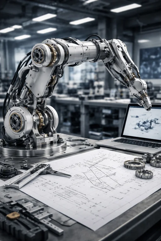
Industrial robotic arm prototype on an engineering workbench with mechanical joints, gears, and digital modeling used in robot kinematics and dynamics.

Multi-Axis Articulated Manipulator Analyzed via Kinematic Transforms and Dynamic Equations of Motion

This physical prototype demonstrates the interaction between geometric kinematics and multi-body dynamics in an articulated robotic manipulator. The serial chain of rigid links and revolute joints is modeled geometrically using Denavit–Hartenberg homogeneous transformations and differential Jacobians. Concurrently, closed-loop model-based controllers rely on the non-linear equations of motion—accounting for configuration-dependent inertia matrices, velocity-dependent Coriolis and centrifugal vectors, and gravitational loading—to command exact motor torques and preserve trajectory tracking fidelity.

Interactive Quick Review: Kinematics vs. Dynamics Fundamentals

Test your understanding of pure geometric motion versus force-driven dynamics before exploring forward kinematics transformations:

1. What is the fundamental distinction between robot kinematics and robot dynamics?

Answer: Kinematics studies pure motion geometry (position, velocity, acceleration, and orientation) without regard to forces, whereas dynamics incorporates mass, link inertia, gravity, and torques to determine the physical forces required to produce motion.

2. What nonlinear mapping does forward kinematics compute in robotic manipulators?

Answer: Forward kinematics computes a non-linear geometric mapping from joint configuration space variables $\mathbf{q} \in \mathbb{R}^n$ (joint angles or prismatic displacements) into Cartesian task space poses $\mathbf{x} \in SE(3)$ of the tool center point.

Glossary of Key Terminology

Essential mathematical concepts governing spatial rigid-body kinematics, velocity mappings, and non-linear manipulator dynamics:

Denavit–Hartenberg (D–H) Convention A standardized geometric convention that attaches reference frames to serial kinematic links using four parameters per joint: link length ($a_i$), link twist ($\alpha_i$), link offset ($d_i$), and joint angle ($\theta_i$).

Manipulator Geometric Jacobian ($\mathbf{J}(\mathbf{q})$) A configuration-dependent sensitivity matrix that maps joint velocity vectors $\dot{\mathbf{q}}$ to the Cartesian linear and angular velocity twist $\mathbf{v}_e = [\dot{\mathbf{p}}_e^T, \boldsymbol{\omega}_e^T]^T$ of the end-effector.

Kinematic Singularity A mechanical configuration $\mathbf{q}$ where the Jacobian matrix drops rank ($\det(\mathbf{J}) = 0$), causing the manipulator to lose instantaneous mobility along one or more Cartesian directions while requiring infinite joint speeds for infinitesimal Cartesian motion.

Euler–Lagrange Equations of Motion An energy-based analytical mechanics formulation defined by $\frac{d}{dt}\left(\frac{\partial L}{\partial \dot{q}_i}\right) - \frac{\partial L}{\partial q_i} = \tau_i$, yielding coupled second-order non-linear differential equations without requiring explicit internal constraint force modeling.

Computed Torque Control (Feedback Linearization) A model-based control strategy that uses dynamic equations in a feedforward loop ($\boldsymbol{\tau} = \mathbf{M}(\mathbf{q})\mathbf{v} + \mathbf{C}(\mathbf{q}, \dot{\mathbf{q}})\dot{\mathbf{q}} + \mathbf{G}(\mathbf{q})$) to cancel non-linearities and decouple the robot into independent linear systems.

Forward Kinematics & Denavit–Hartenberg Parameters

Forward kinematics determines the spatial pose (position and orientation) of a robot's end-effector relative to a fixed base reference frame from given joint values $\mathbf{q} = [q_1, q_2, \dots, q_n]^T$. Mathematically, it defines a continuous mapping $\mathbf{f}: \mathcal{Q} \to SE(3)$.

For an $n$-link serial manipulator, the compound homogeneous transformation matrix from base frame 0 to tool frame $n$ is the ordered product of link transforms:

$$\mathbf{T}_0^n(\mathbf{q}) = \mathbf{A}_1(q_1) \mathbf{A}_2(q_2) \dots \mathbf{A}_n(q_n)$$

The standard Denavit–Hartenberg (D–H) convention systematically constructs each link transformation matrix $\mathbf{A}_i$ via four successive transformations about link axes:

$$\mathbf{A}_i = \text{Rot}_{z, \theta_i} \, \text{Trans}_{z, d_i} \, \text{Trans}_{x, a_i} \, \text{Rot}_{x, \alpha_i}$$

Expanding the matrix product yields the standardized $4 \times 4$ link transformation:

$$\mathbf{A}_i = \begin{bmatrix} \cos\theta_i & -\sin\theta_i \cos\alpha_i & \sin\theta_i \sin\alpha_i & a_i \cos\theta_i \\ \sin\theta_i & \cos\theta_i \cos\alpha_i & -\cos\theta_i \sin\alpha_i & a_i \sin\theta_i \\ 0 & \sin\alpha_i & \cos\alpha_i & d_i \\ 0 & 0 & 0 & 1 \end{bmatrix}$$

The four parameters are defined as:

Link length ($a_i$): Distance between axis $z_{i-1}$ and axis $z_i$ along common normal $x_i$.
Link twist ($\alpha_i$): Angle from axis $z_{i-1}$ to axis $z_i$ measured about $x_i$.
Link offset ($d_i$): Distance from origin $O_{i-1}$ to common normal intersection along axis $z_{i-1}$ (variable for prismatic joints).
Joint angle ($\theta_i$): Rotation from axis $x_{i-1}$ to axis $x_i$ about axis $z_{i-1}$ (variable for revolute joints).

Homogeneous Transformations: Structural Anatomy of R and p

To fully describe spatial transformations on manifolds, robotics represents rigid-body poses within the Special Euclidean group $SE(3)$ using a $4 \times 4$ homogeneous transformation matrix:

$$\mathbf{T} = \begin{bmatrix} \mathbf{R} & \mathbf{p} \\ \mathbf{0}_{1 \times 3} & 1 \end{bmatrix} = \begin{bmatrix} r_{11} & r_{12} & r_{13} & p_x \\ r_{21} & r_{22} & r_{23} & p_y \\ r_{31} & r_{32} & r_{33} & p_z \\ 0 & 0 & 0 & 1 \end{bmatrix}$$

The transformation partitions cleanly into functional blocks:

Translation Vector ($\mathbf{p} \in \mathbb{R}^3$): Explicit displacement vector connecting the origin of the base frame to the origin of the target frame.
Rotation Matrix ($\mathbf{R} \in SO(3)$): Orthogonal matrix satisfying $\mathbf{R}^T \mathbf{R} = \mathbf{I}$ and $\det(\mathbf{R}) = +1$. The column vectors $\mathbf{r}_1, \mathbf{r}_2, \mathbf{r}_3$ represent unit basis vectors of the transformed frame expressed in base coordinates: $$\mathbf{R} = \begin{bmatrix} \mathbf{n} & \mathbf{s} & \mathbf{a} \end{bmatrix} = \begin{bmatrix} \hat{\mathbf{x}}_1^0 & \hat{\mathbf{y}}_1^0 & \hat{\mathbf{z}}_1^0 \end{bmatrix}$$

Transforming a point vector $\mathbf{x}_1$ from Frame 1 to Frame 0 is calculated via affine mapping:

$$\mathbf{x}_0 = \mathbf{R} \mathbf{x}_1 + \mathbf{p}$$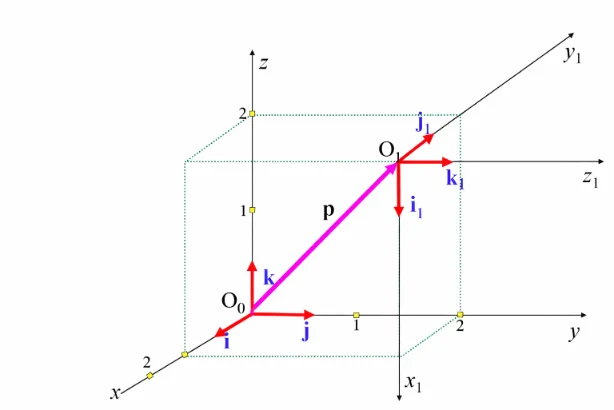

Homogeneous transformation example showing two coordinate frames where the second frame is translated by (1, 2, 2) from the original origin and rotated so that its x-axis aligns with the positive y-direction, its y-axis aligns with the negative z-direction, and its z-axis aligns with the negative x-direction.

Spatial Transformation Between Coordinate Frames Featuring Combined Translation and Axis Rotation

Inverse Kinematics & Numerical Solvers

Inverse kinematics computes the joint vector $\mathbf{q}$ corresponding to a desired end-effector pose $\mathbf{x}_d \in SE(3)$:

$$\mathbf{q} = \mathbf{f}^{-1}(\mathbf{x}_d)$$

Unlike forward kinematics, inverse kinematics problems are non-linear and coupled. They may possess closed-form analytical solutions (satisfying the Pieper criterion for 6-DOF arms with three intersecting wrist axes), multiple discrete solutions (e.g., elbow-up versus elbow-down configurations), or infinite solutions in kinematically redundant arms.

For general geometries without closed-form formulations, solutions are evaluated iteratively via the Newton-Raphson update:

$$\mathbf{q}_{k+1} = \mathbf{q}_k + \mathbf{J}^\dagger(\mathbf{q}_k) \left( \mathbf{x}_d - \mathbf{f}(\mathbf{q}_k) \right)$$

where $\mathbf{J}^\dagger = \mathbf{J}^T (\mathbf{J} \mathbf{J}^T)^{-1}$ denotes the Moore-Penrose pseudo-inverse.

Differential Kinematics & The Manipulator Jacobian

The geometric Jacobian matrix $\mathbf{J}(\mathbf{q}) \in \mathbb{R}^{6 \times n}$ maps joint velocity space to Cartesian operational velocity space:

$$\mathbf{v}_e = \begin{bmatrix} \dot{\mathbf{p}}_e \\ \boldsymbol{\omega}_e \end{bmatrix} = \mathbf{J}(\mathbf{q}) \dot{\mathbf{q}} = \begin{bmatrix} \mathbf{J}_1 & \mathbf{J}_2 & \dots & \mathbf{J}_n \end{bmatrix} \dot{\mathbf{q}}$$

The individual column vectors $\mathbf{J}_i$ for joint $i$ are constructed geometrically:

$$\mathbf{J}_i = \begin{cases} \begin{bmatrix} \mathbf{z}_{i-1} \times (\mathbf{p}_e - \mathbf{p}_{i-1}) \\ \mathbf{z}_{i-1} \end{bmatrix} & \text{(Revolute Joint)} \\[10pt] \begin{bmatrix} \mathbf{z}_{i-1} \\ \mathbf{0}_{3 \times 1} \end{bmatrix} & \text{(Prismatic Joint)} \end{cases}$$

where $\mathbf{z}_{i-1}$ is the unit vector along joint axis $i$, $\mathbf{p}_{i-1}$ is the origin of frame $i-1$, and $\mathbf{p}_e$ is the position of the tool center point.

Static Force Duality via Virtual Work

By the principle of virtual work, lossless power conservation between joint space and operational space demands:

$$\delta W = \boldsymbol{\tau}^T \delta \mathbf{q} - \mathbf{F}_e^T \delta \mathbf{x} = 0$$

Substituting $\delta \mathbf{x} = \mathbf{J}(\mathbf{q}) \delta \mathbf{q}$ yields the static force transmission relation:

$$\boldsymbol{\tau} = \mathbf{J}^T(\mathbf{q}) \mathbf{F}_e$$

where $\mathbf{F}_e = [\mathbf{f}_e^T, \mathbf{m}_e^T]^T$ represents Cartesian forces and moments exerted by the end-effector.

Kinematic Singularities & Inversion Regularization

Singular configurations occur where $\det(\mathbf{J}(\mathbf{q})) = 0$, causing rank loss and infinite joint velocity demands near the singular direction. To maintain stability near singular configurations during numerical inversion, controllers utilize the Damped Least Squares (Levenberg-Marquardt) pseudoinverse:

$$\mathbf{J}^* = \mathbf{J}^T \left( \mathbf{J} \mathbf{J}^T + \lambda^2 \mathbf{I} \right)^{-1}$$

where $\lambda > 0$ is a damping factor bounding peak joint velocities at the cost of bounded Cartesian tracking error.

Engineering Challenges & Technical Solutions

Implementing kinematics and dynamic equations on real-world industrial manipulators introduces several practical electromechanical challenges:

1. Kinematic Singularities and Actuator Velocity Saturation

The Challenge: When an arm approaches boundary or internal singularities (e.g., wrist alignments, fully extended elbows), inverting the Jacobian ($\dot{\mathbf{q}} = \mathbf{J}^{-1}\mathbf{v}$) demands near-infinite joint speeds. This causes actuator over-current trips, motor saturation, and severe tracking deviation.

Technical Solutions:

Singularity-Robust Damped Least Squares: Adding a damping factor $\lambda$ dynamically scaled by manipulability index $w = \sqrt{\det(\mathbf{J}\mathbf{J}^T)}$, bounding maximum commanded joint velocities.
Task-Priority Redundancy Resolution: Exploiting 7-DOF null-space projections ($\dot{\mathbf{q}} = \mathbf{J}^\dagger \mathbf{v} + (\mathbf{I} - \mathbf{J}^\dagger \mathbf{J})\dot{\mathbf{q}}_0$) to reconfigure joint postures away from singular boundaries while maintaining the primary tool path.

2. Dynamic Parameter Uncertainty and Payload Shifts

The Challenge: Model-based controllers rely on precise link masses, centers of gravity, and inertia tensors. Grasping unmodeled payloads or handling variations in manufactured components causes mismatch between actual dynamics and the feedforward model, leading to tracking errors.

Technical Solutions:

Online Recursive Least Squares (RLS) Parameter Identification: Exploiting the linear-in-the-parameters property of robot dynamics ($\boldsymbol{\tau} = \mathbf{Y}(\mathbf{q}, \dot{\mathbf{q}}, \ddot{\mathbf{q}})\boldsymbol{\theta}$) to estimate unknown payload mass and inertia parameters during operation.
Adaptive Slotine-Li Control: Updating dynamic estimates in real time using tracking error feedback, guaranteeing asymptotic convergence without requiring joint acceleration measurements.

3. Unmodeled Joint Friction and Gear Backlash

The Challenge: Harmonic drive gearboxes, cycloidal drives, and bearings exhibit non-linear friction (Coulomb, static stiction, viscous friction, Stribeck curves) and structural flexibility, degrading low-velocity tracking performance.

Technical Solutions:

Model-Based Feedforward Friction Compensation: Augmenting the control law with dynamic friction models: $\boldsymbol{\tau}_{\text{fric}} = \mathbf{F}_v \dot{\mathbf{q}} + \mathbf{F}_c \text{sgn}(\dot{\mathbf{q}})$.
Dual-Encoder Systems: Placing high-resolution absolute optical encoders on both motor inputs and gearbox output shafts to monitor and compensate for mechanical backlash and compliance directly.

4. Multi-Axis Dynamic Coupling in High-Speed Manipulation

The Challenge: At high accelerations, off-diagonal inertia terms $m_{ij}(\mathbf{q})$ and velocity-squared Coriolis forces $C_{ijk}\dot{q}_j \dot{q}_k$ induce torques across adjacent joints. Uncompensated coupling creates trajectory errors that single-joint PID controllers cannot suppress.

Technical Solutions:

Full Computed Torque Control: Evaluating the complete multi-body dynamic equations in real time to cancel coupling torques via feedforward compensation, as discussed in Advanced Control Systems in Robotics.
High Gear Ratio Transmission: Using gear reductions ($N > 100$) to scale motor rotor inertia by $N^2$, which reduces the relative effect of dynamic cross-coupling across links.

Multi-Body Dynamic Equations of Motion

The matrix dynamic equation of an $n$-link articulated rigid manipulator is formulated compactly as:

$$\mathbf{M}(\mathbf{q})\ddot{\mathbf{q}} + \mathbf{C}(\mathbf{q}, \dot{\mathbf{q}})\dot{\mathbf{q}} + \mathbf{G}(\mathbf{q}) = \boldsymbol{\tau} - \mathbf{J}^T(\mathbf{q})\mathbf{F}_e$$

where:

$\mathbf{M}(\mathbf{q}) \in \mathbb{R}^{n \times n}$: Configuration-dependent, symmetric, positive-definite Generalized Inertia Matrix satisfying $\mathbf{M}(\mathbf{q}) = \mathbf{M}^T(\mathbf{q}) > 0$.
$\mathbf{C}(\mathbf{q}, \dot{\mathbf{q}})\dot{\mathbf{q}} \in \mathbb{R}^n$: Centrifugal and Coriolis torque vector, derived from Christoffel symbols of the first kind: $$c_{ij} = \sum_{k=1}^{n} \Gamma_{ijk} \dot{q}_k = \frac{1}{2} \sum_{k=1}^{n} \left( \frac{\partial m_{ij}}{\partial q_k} + \frac{\partial m_{ik}}{\partial q_j} - \frac{\partial m_{jk}}{\partial q_i} \right) \dot{q}_k$$
$\mathbf{G}(\mathbf{q}) \in \mathbb{R}^n$: Conservative gravitational torque vector, derived from potential energy: $\mathbf{G}(\mathbf{q}) = \frac{\partial V(\mathbf{q})}{\partial \mathbf{q}}$.
$\boldsymbol{\tau} \in \mathbb{R}^n$: Commanded generalized joint actuator torque vector.

A key property of this formulation is the skew-symmetry of the matrix $\dot{\mathbf{M}}(\mathbf{q}) - 2\mathbf{C}(\mathbf{q}, \dot{\mathbf{q}})$, which ensures workless Coriolis forces and guarantees passivity:

$$\mathbf{x}^T \left( \dot{\mathbf{M}}(\mathbf{q}) - 2\mathbf{C}(\mathbf{q}, \dot{\mathbf{q}}) \right) \mathbf{x} = 0 \quad \forall \mathbf{x} \in \mathbb{R}^n$$

Interactive Quick Review: Singularities, Euler-Lagrange & Force Mapping

Reinforce key concepts regarding Jacobian singularities, virtual work force mapping, and Lagrangian dynamics before reviewing the FAQ:

1. How does the transpose of the Jacobian matrix ($\mathbf{J}^T$) relate Cartesian end-effector forces ($\mathbf{F}$) to joint torques ($\boldsymbol{\tau}$)?

Answer: Via the principle of virtual work: $\boldsymbol{\tau} = \mathbf{J}^T \mathbf{F}$, where $\mathbf{J}^T$ maps static Cartesian forces and moments exerted at the tool tip directly into equivalent static joint actuator torques.

2. What physical phenomenon occurs when a manipulator reaches a kinematic singularity ($\det(\mathbf{J}) = 0$)?

Answer: The robot loses one or more degrees of freedom in Cartesian space, requiring infinitely large joint velocities to move along the lost direction and rendering analytical inversion ($\mathbf{J}^{-1}$) impossible.

External References and Further Reading

To explore rigid-body kinematics, Denavit–Hartenberg conventions, and manipulator dynamics theory, consult the following authoritative sources:

Robot Modeling and Control (Spong, Hutchinson, Vidyasagar) – A foundational textbook offering rigorous mathematical treatments of D–H parameters, Jacobians, and Euler-Lagrange dynamics.
Robotics: Modelling, Planning and Control (Siciliano et al.) – Comprehensive academic reference covering forward/inverse kinematics, operational space dynamics, and singularity analysis.
IEEE Robotics and Automation Society (RAS) – Global professional organization publishing peer-reviewed research on robot kinematics, dynamic modeling, and industrial manipulator control.

Frequently Asked Questions about Robot Kinematics and Dynamics

What is the Denavit–Hartenberg (D–H) convention, and why is it useful?

The D–H convention is a standardized mathematical framework that uses four parameters per joint (link length $a_i$, twist $\alpha_i$, offset $d_i$, and angle $\theta_i$) to attach coordinate frames to robot links, allowing systematic construction of homogeneous transformation matrices.

Why is inverse kinematics significantly harder to solve than forward kinematics?

Forward kinematics involves straightforward sequential matrix multiplication ($\mathbf{T} = \mathbf{A}_1 \mathbf{A}_2 \dots \mathbf{A}_n$). Inverse kinematics requires solving a system of non-linear trigonometric equations ($\mathbf{q} = \mathbf{f}^{-1}(\mathbf{x})$), which can yield zero, multiple, or infinite solutions.

What is the geometrical interpretation of the columns of a 3 × 3 rotation matrix R?

The three columns of $\mathbf{R}$ represent unit vectors defining the orientation of the transformed frame's x, y, and z axes expressed in the coordinates of the base reference frame.

How does the Jacobian matrix change with robot posture q?

Because link positions and joint axes shift in space as the arm moves, the entries of $\mathbf{J}(\mathbf{q})$ are non-linear trigonometric functions of joint positions $\mathbf{q}$. Consequently, the robot's velocity sensitivity and force transmission change continuously across its workspace.

What causes dynamic coupling between robot arm joints?

Off-diagonal terms $m_{ij}(\mathbf{q})$ in the inertia matrix $\mathbf{M}(\mathbf{q})$ represent dynamic coupling. Accelerating joint $i$ generates inertial reaction forces that physically induce torques in joint $j$, even if joint $j$ is commanded to hold still.

How does computed torque control linearize robot arm dynamics?

Computed torque control uses the inverse dynamic model ($\boldsymbol{\tau} = \mathbf{M}(\mathbf{q})\mathbf{v} + \mathbf{C}(\mathbf{q}, \dot{\mathbf{q}})\dot{\mathbf{q}} + \mathbf{G}(\mathbf{q})$) in feedforward loops to algebraically cancel non-linear Coriolis, centrifugal, and gravitational forces, simplifying control to linear acceleration loops ($\mathbf{v}$).

End-of-Page Exercises: Review, Thought-Provoking & Engineering Problems

Section 1: Foundational Review Questions & Answers

1. What four parameters define a Denavit–Hartenberg joint transformation?

Answer: Link length ($a_i$), link twist ($\alpha_i$), link offset ($d_i$), and joint angle ($\theta_i$).

2. What is the mathematical structure of a 4 × 4 homogeneous transformation matrix T?

Answer: An upper-left $3 \times 3$ rotation matrix $\mathbf{R}$, an upper-right $3 \times 1$ translation vector $\mathbf{p}$, a lower-left $1 \times 3$ zero row vector, and a bottom-right scalar 1.

3. What property of rotation matrices makes matrix inversion equal to the transpose ($\mathbf{R}^{-1} = \mathbf{R}^T$)?

Answer: Orthogonality (since $\mathbf{R} \in SO(3)$, its columns form an orthonormal basis: $\mathbf{R}^T \mathbf{R} = \mathbf{I}$).

4. How does the Jacobian matrix $\mathbf{J}(\mathbf{q})$ relate joint velocities $\dot{\mathbf{q}}$ to Cartesian velocity $\mathbf{v}_e$?

Answer: Through the linear differential mapping $\mathbf{v}_e = \mathbf{J}(\mathbf{q})\dot{\mathbf{q}}$.

5. What condition defines a kinematic singularity in terms of the Jacobian determinant?

Answer: $\det(\mathbf{J}(\mathbf{q})) = 0$, indicating loss of matrix rank and the loss of Cartesian mobility along at least one direction.

6. What is the fundamental matrix dynamic equation governing an n-link robotic manipulator?

Answer: $\mathbf{M}(\mathbf{q})\ddot{\mathbf{q}} + \mathbf{C}(\mathbf{q}, \dot{\mathbf{q}})\dot{\mathbf{q}} + \mathbf{G}(\mathbf{q}) = \boldsymbol{\tau}$.

7. What physical property is described by the off-diagonal terms of the inertia matrix $\mathbf{M}(\mathbf{q})$?

Answer: Dynamic inertial cross-coupling, indicating how angular acceleration at joint $i$ physically induces an inertial reaction torque at joint $j$.

8. How is the Lagrangian L defined in energy-based robot dynamic modeling?

Answer: $L = T - V$, representing the difference between total system kinetic energy $T$ and potential energy $V$.

9. What formula maps end-effector Cartesian force F to joint torques $\boldsymbol{\tau}$?

Answer: $\boldsymbol{\tau} = \mathbf{J}^T(\mathbf{q})\mathbf{F}$, derived from the principle of virtual work.

10. Name four mathematical subjects required for mastering robot kinematics and dynamics.

Answer: Linear algebra, multivariable calculus, differential equations, and classical analytical mechanics.

Section 2: Analytical & Thought-Provoking Questions

1. Why do small numerical errors in joint encoder readings propagate non-linearly into large Cartesian positioning errors at the end-effector?

Answer: Forward kinematics compounds transformations ($\mathbf{T} = \mathbf{A}_1 \mathbf{A}_2 \dots \mathbf{A}_n$). Angular joint errors $\Delta \theta_i$ act across link lengths $L_i$, producing tip displacements $\Delta x \approx L_i \Delta \theta_i$. In long serial chains, angular errors at base joints amplify linearly with arm length, while rotary matrix multiplications introduce cumulative trigonometric coupling.

2. How does operating near a kinematic singularity destabilize velocity-based joint controllers?

Answer: Velocity control computes joint speeds via $\dot{\mathbf{q}} = \mathbf{J}^{-1}(\mathbf{q}) \mathbf{v}$. Near singularities, $\det(\mathbf{J}) \to 0$, causing elements of $\mathbf{J}^{-1}$ to approach infinity. Demanding even a small Cartesian tool velocity near a singularity forces the controller to demand unachievable joint speeds, leading to actuator saturation, over-speed trips, or violent structural vibrations.

3. Why does an unmodeled payload mass held at the gripper degrade computed torque control performance?

Answer: Computed torque feedforward ($\boldsymbol{\tau} = \mathbf{M}(\mathbf{q})\mathbf{v} + \mathbf{C}\dot{\mathbf{q}} + \mathbf{G}$) relies on accurate link mass parameters. An unmodeled payload shifts the center of mass and increases actual inertia ($\mathbf{M}_{\text{real}} > \mathbf{M}_{\text{model}}$) and gravity torques ($\mathbf{G}_{\text{real}} > \mathbf{G}_{\text{model}}$), leading to feedforward torque under-prediction and persistent trajectory tracking lag.

4. What is the physical mechanism behind Coriolis forces $\mathbf{C}(\mathbf{q}, \dot{\mathbf{q}})\dot{\mathbf{q}}$ in multi-link rotational manipulators?

Answer: Coriolis forces arise when a body translates within a rotating reference frame. In a 2-link arm, extending Link 2 radially while Link 1 rotates changes the effective radial distance of Link 2's mass from the shoulder axis, generating cross-coupled reaction torques proportional to the product of joint velocities ($\dot{\theta}_1 \dot{\theta}_2$).

5. Why are 7-DOF serial manipulators termed kinematically redundant, and how do they benefit obstacle avoidance?

Answer: Specifying an end-effector pose in 3D space requires 6 degrees of freedom. A 7-DOF arm possesses one redundant degree of freedom ($7 - 6 = 1$), creating a continuous 1D self-motion null-space manifold for a fixed end-effector pose. The controller can swivel the elbow link to dodge obstacles without perturbing the end-effector trajectory.

6. How does the principle of virtual work establish the static force duality $\boldsymbol{\tau} = \mathbf{J}^T \mathbf{F}$?

Answer: Virtual work requires that work performed in joint space ($\delta W = \boldsymbol{\tau}^T \delta \mathbf{q}$) equals work in Cartesian space ($\delta W = \mathbf{F}^T \delta \mathbf{x}$) under static equilibrium. Substituting $\delta \mathbf{x} = \mathbf{J}\delta \mathbf{q}$ yields $\boldsymbol{\tau}^T \delta \mathbf{q} = \mathbf{F}^T \mathbf{J} \delta \mathbf{q}$. Taking the transpose confirms $\boldsymbol{\tau} = \mathbf{J}^T \mathbf{F}$.

7. Why is the inertia matrix $\mathbf{M}(\mathbf{q})$ guaranteed to be symmetric and positive-definite?

Answer: Kinetic energy is a strictly positive physical scalar ($T = \frac{1}{2}\dot{\mathbf{q}}^T \mathbf{M}(\mathbf{q})\dot{\mathbf{q}} > 0$ for all non-zero velocities $\dot{\mathbf{q}} \neq \mathbf{0}$), requiring $\mathbf{M}(\mathbf{q})$ to be positive-definite. Symmetry ($m_{ij} = m_{ji}$) reflects reciprocal inertial coupling between joint linkages governed by Newton's third law.

8. How does numerical Newton-Raphson inverse kinematics resolve joint targets when closed-form equations are unavailable?

Answer: The algorithm linearizes forward kinematics iteratively via $\mathbf{q}_{k+1} = \mathbf{q}_k + \mathbf{J}^\dagger(\mathbf{q}_k)(\mathbf{x}_d - \mathbf{f}(\mathbf{q}_k))$. At each iteration, it computes Cartesian error, multiplies by the Jacobian pseudoinverse to calculate joint increments $\Delta \mathbf{q}$, and updates the configuration estimate until error norms drop below an assigned tolerance.

9. Why do direction cosine matrices R require six constraint equations to represent three rotational degrees of freedom?

Answer: A $3 \times 3$ matrix contains nine scalar entries. Orthogonality demands that the three columns are unit vectors ($\|\mathbf{r}_i\| = 1$, providing 3 constraints) and mutually perpendicular ($\mathbf{r}_i \cdot \mathbf{r}_j = 0$ for $i \neq j$, providing 3 constraints). Subtracting 6 constraints from 9 elements leaves exactly 3 independent rotational degrees of freedom.

10. How does high gear reduction (N > 100:1) in industrial actuators mask dynamic link coupling effects?

Answer: High gear ratios scale reflected motor rotor inertia by $N^2$ at the joint. When $N$ is large, the rotor inertia dominates the dynamic equation, making off-diagonal link coupling terms $m_{ij}(\mathbf{q})$ small relative to actuator inertia, enabling decoupled single-joint PID control.

11. Why do SCARA robots feature constant gravity torques G(q) = 0 across all joint configurations during horizontal motion?

Answer: SCARA revolute joint axes are aligned vertically, parallel to the gravity vector. Because link rotations occur in horizontal planes perpendicular to gravity, joint movements produce zero vertical displacement of link centers of mass, rendering potential energy constant ($\partial V / \partial q_i = 0$) and gravitational torque zero.

12. How does gravity vector rotation account for mounting an industrial robot on an inclined wall or ceiling?

Answer: Gravitational torques $\mathbf{G}(\mathbf{q})$ depend on the orientation of the base frame relative to the world gravity vector $\mathbf{g}$. Mounting the robot on an inclined or inverted surface changes the direction of $\mathbf{g}$ in base coordinates; the controller must update its internal gravity model, or feedforward torques will act in the wrong direction.

Section 3: Numerical Engineering Problems & Solutions

Problem 1: Homogeneous Transformation Vector Mapping
A point $\mathbf{x}_1 = [2.0, 0.0, 1.0]^T\text{ meters}$ is expressed in Frame 1. Frame 1 is related to Frame 0 by the homogeneous transformation matrix: $$\mathbf{T}_0^1 = \begin{bmatrix} 0 & -1 & 0 & 3.0 \\ 1 & 0 & 0 & 1.0 \\ 0 & 0 & 1 & 4.0 \\ 0 & 0 & 0 & 1.0 \end{bmatrix}$$ Calculate the coordinates of the mapped point $\mathbf{x}_0 = [x_0, y_0, z_0]^T$ expressed in Frame 0.

Solution:
1. Apply the transformation equation $\mathbf{x}_0 = \mathbf{R} \mathbf{x}_1 + \mathbf{p}$: $$\mathbf{R}\mathbf{x}_1 = \begin{bmatrix} 0 & -1 & 0 \\ 1 & 0 & 0 \\ 0 & 0 & 1 \end{bmatrix} \begin{bmatrix} 2.0 \\ 0.0 \\ 1.0 \end{bmatrix} = \begin{bmatrix} (0)(2.0) + (-1)(0.0) + (0)(1.0) \\ (1)(2.0) + (0)(0.0) + (0)(1.0) \\ (0)(2.0) + (0)(0.0) + (1)(1.0) \end{bmatrix} = \begin{bmatrix} 0.0 \\ 2.0 \\ 1.0 \end{bmatrix}$$ 2. Add the translation vector $\mathbf{p} = [3.0, 1.0, 4.0]^T$: $$\mathbf{x}_0 = \begin{bmatrix} 0.0 \\ 2.0 \\ 1.0 \end{bmatrix} + \begin{bmatrix} 3.0 \\ 1.0 \\ 4.0 \end{bmatrix} = \begin{bmatrix} 3.0 \\ 3.0 \\ 5.0 \end{bmatrix}\text{ meters}$$ Final Answer: Transformed coordinates in Frame 0 are $\mathbf{x}_0 = [3.0, 3.0, 5.0]^T\text{ meters}$.

Problem 2: 2-Link Planar Forward Kinematics Computation
A 2-link planar arm has link lengths $L_1 = 0.8\text{ m}$ and $L_2 = 0.6\text{ m}$. The joint angles are set to $\theta_1 = 30^\circ$ and $\theta_2 = 45^\circ$ ($\theta_1 + \theta_2 = 75^\circ$). Calculate the Cartesian coordinates $(x, y)$ of the end-effector in meters. (Given: $\cos 30^\circ \approx 0.8660$, $\sin 30^\circ = 0.5000$, $\cos 75^\circ \approx 0.2588$, $\sin 75^\circ \approx 0.9659$).

Solution:
1. Calculate $x$-coordinate: $$x = L_1 \cos\theta_1 + L_2 \cos(\theta_1 + \theta_2) = (0.8 \times 0.8660) + (0.6 \times 0.2588) = 0.6928 + 0.1553 = 0.8481\text{ m}$$ 2. Calculate $y$-coordinate: $$y = L_1 \sin\theta_1 + L_2 \sin(\theta_1 + \theta_2) = (0.8 \times 0.5000) + (0.6 \times 0.9659) = 0.4000 + 0.5795 = 0.9795\text{ m}$$ Final Answer: End-effector coordinates are $x = 0.85\text{ m}$ and $y = 0.98\text{ m}$.

Problem 3: Jacobian Determinant Singularity Condition
A planar 2-link robot has link lengths $L_1 = 0.5\text{ m}$ and $L_2 = 0.4\text{ m}$. Its Jacobian determinant is given by $\det(\mathbf{J}) = L_1 L_2 \sin\theta_2$. Calculate $\det(\mathbf{J})$ for joint angles $\theta_2 = 90^\circ$ ($\sin 90^\circ = 1.0$) and $\theta_2 = 0^\circ$ ($\sin 0^\circ = 0$), identifying which posture is singular.

Solution:
1. Evaluate at $\theta_2 = 90^\circ$: $$\det(\mathbf{J}) = 0.5 \times 0.4 \times 1.0 = 0.20\text{ m}^2 \quad (\det(\mathbf{J}) \neq 0 \Rightarrow \text{Non-singular})$$ 2. Evaluate at $\theta_2 = 0^\circ$: $$\det(\mathbf{J}) = 0.5 \times 0.4 \times 0.0 = 0.00\text{ m}^2 \quad (\det(\mathbf{J}) = 0 \Rightarrow \text{Singular})$$ Final Answer: At $\theta_2 = 90^\circ$, $\det(\mathbf{J}) = \mathbf{0.20\text{ m}^2}$; at $\theta_2 = 0^\circ$, $\det(\mathbf{J}) = \mathbf{0.00}$, confirming a boundary kinematic singularity.

Problem 4: Jacobian Velocity Mapping Calculation
At a specific joint posture, a 2-link manipulator has the evaluated Jacobian matrix: $$\mathbf{J} = \begin{bmatrix} -0.4 & -0.2 \\ 0.7 & 0.3 \end{bmatrix}\text{ m/rad}$$ If joint velocities are commanded as $\dot{\mathbf{q}} = [\dot{\theta}_1, \dot{\theta}_2]^T = [2.0, -1.0]^T\text{ rad/s}$, calculate the resulting Cartesian tool velocity vector $[\dot{x}, \dot{y}]^T$ in meters per second.

Solution:
1. Apply the differential mapping $\mathbf{v} = \mathbf{J} \dot{\mathbf{q}}$: $$\dot{x} = (-0.4 \times 2.0) + (-0.2 \times -1.0) = -0.8 + 0.2 = -0.60\text{ m/s}$$ $$\dot{y} = (0.7 \times 2.0) + (0.3 \times -1.0) = 1.4 - 0.3 = 1.10\text{ m/s}$$ Final Answer: Cartesian end-effector velocity is $[\dot{x}, \dot{y}]^T = [-0.60, 1.10]^T\text{ m/s}$.

Problem 5: Static Force Transpose Mapping ($\boldsymbol{\tau} = \mathbf{J}^T \mathbf{F}$)
A robot tool tip exerts a Cartesian force vector $\mathbf{F} = [F_x, F_y]^T = [10.0, -20.0]^T\text{ N}$ against an environmental surface. The Jacobian matrix at this configuration is: $$\mathbf{J} = \begin{bmatrix} -0.3 & -0.1 \\ 0.5 & 0.2 \end{bmatrix}$$ Compute the Jacobian transpose $\mathbf{J}^T$ and calculate the required static joint torques $\boldsymbol{\tau} = [\tau_1, \tau_2]^T$ in Newton-meters.

Solution:
1. Form the transpose matrix: $$\mathbf{J}^T = \begin{bmatrix} -0.3 & 0.5 \\ -0.1 & 0.2 \end{bmatrix}$$ 2. Compute torque for joint 1: $$\tau_1 = (-0.3 \times 10.0) + (0.5 \times -20.0) = -3.0 - 10.0 = -13.0\text{ N}\cdot\text{m}$$ 3. Compute torque for joint 2: $$\tau_2 = (-0.1 \times 10.0) + (0.2 \times -20.0) = -1.0 - 4.0 = -5.0\text{ N}\cdot\text{m}$$ Final Answer: Required static torques are $\tau_1 = -13.0\text{ N}\cdot\text{m}$ and $\tau_2 = -5.0\text{ N}\cdot\text{m}$.

Problem 6: Dynamic Joint Coupling Torque Matrix Product
A 2-link manipulator inertia matrix is given by: $$\mathbf{M}(\mathbf{q}) = \begin{bmatrix} 1.5 & 0.4 \\ 0.4 & 0.6 \end{bmatrix}\text{ kg}\cdot\text{m}^2$$ If desired joint accelerations are $\ddot{\mathbf{q}} = [\ddot{q}_1, \ddot{q}_2]^T = [3.0, -2.0]^T\text{ rad/s}^2$, calculate the inertial joint torque vector $\boldsymbol{\tau}_{\text{inertia}} = \mathbf{M}(\mathbf{q})\ddot{\mathbf{q}}$ in Newton-meters.

Solution:
1. Compute inertial torque for joint 1: $$\tau_1 = (1.5 \times 3.0) + (0.4 \times -2.0) = 4.5 - 0.8 = 3.7\text{ N}\cdot\text{m}$$ 2. Compute inertial torque for joint 2: $$\tau_2 = (0.4 \times 3.0) + (0.6 \times -2.0) = 1.2 - 1.2 = 0.0\text{ N}\cdot\text{m}$$ Final Answer: Inertial torque vector is $\boldsymbol{\tau}_{\text{inertia}} = [3.7, 0.0]^T\text{ N}\cdot\text{m}$.

Problem 7: Kinetic Energy Calculation from Inertia Matrix
For a manipulator with inertia matrix $\mathbf{M}(\mathbf{q}) = \begin{bmatrix} 2.0 & 0.5 \\ 0.5 & 1.0 \end{bmatrix}\text{ kg}\cdot\text{m}^2$, calculate total system kinetic energy $T = \frac{1}{2}\dot{\mathbf{q}}^T \mathbf{M}(\mathbf{q})\dot{\mathbf{q}}$ when joint velocities are $\dot{\mathbf{q}} = [2.0, 1.0]^T\text{ rad/s}$.

Solution:
1. Compute matrix-vector product $\mathbf{M}(\mathbf{q})\dot{\mathbf{q}}$: $$\mathbf{M}\dot{\mathbf{q}} = \begin{bmatrix} (2.0)(2.0) + (0.5)(1.0) \\ (0.5)(2.0) + (1.0)(1.0) \end{bmatrix} = \begin{bmatrix} 4.0 + 0.5 \\ 1.0 + 1.0 \end{bmatrix} = \begin{bmatrix} 4.5 \\ 2.0 \end{bmatrix}$$ 2. Compute quadratic form $\dot{\mathbf{q}}^T (\mathbf{M}\dot{\mathbf{q}})$: $$\dot{\mathbf{q}}^T (\mathbf{M}\dot{\mathbf{q}}) = (2.0 \times 4.5) + (1.0 \times 2.0) = 9.0 + 2.0 = 11.0\text{ Joules}$$ 3. Scale by $\frac{1}{2}$: $$T = \frac{1}{2} \times 11.0 = 5.5\text{ Joules}$$ Final Answer: Total system kinetic energy is $T = 5.5\text{ Joules}$.

Problem 8: Computed Torque Control Feedforward Sum
A single joint actuator dynamic model requires inertial torque $\mathbf{M}(q)v = 2.4\text{ N}\cdot\text{m}$, Coriolis torque $\mathbf{C}(q, \dot{q})\dot{q} = 0.6\text{ N}\cdot\text{m}$, and gravity torque $\mathbf{G}(q) = 1.8\text{ N}\cdot\text{m}$ at a specific control cycle. Calculate the total required computed torque $\tau = \mathbf{M}(q)v + \mathbf{C}(q, \dot{q})\dot{q} + \mathbf{G}(q)$.

Solution:
1. Sum individual dynamic components: $$\tau = 2.4\text{ N}\cdot\text{m} + 0.6\text{ N}\cdot\text{m} + 1.8\text{ N}\cdot\text{m} = 4.8\text{ N}\cdot\text{m}$$ Final Answer: Total computed feedforward torque is $\tau = 4.8\text{ N}\cdot\text{m}$.

Problem 9: Numerical Inverse Kinematics Error Step Update
A numerical IK solver evaluates joint state $\mathbf{q}_k = [0.50, 0.80]^T\text{ rad}$, with inverted Jacobian: $$\mathbf{J}^{-1}(\mathbf{q}_k) = \begin{bmatrix} 1.2 & -0.4 \\ 0.2 & 0.8 \end{bmatrix}$$ The Cartesian pose error vector is $(\mathbf{x}_d - \mathbf{x}_k) = [0.05, -0.10]^T\text{ meters}$. Calculate the joint update step $\Delta \mathbf{q} = \mathbf{J}^{-1} \Delta \mathbf{x}$ and the updated joint estimate $\mathbf{q}_{k+1} = \mathbf{q}_k + \Delta \mathbf{q}$.

Solution:
1. Calculate joint increment $\Delta \mathbf{q}$: $$\Delta q_1 = (1.2 \times 0.05) + (-0.4 \times -0.10) = 0.06 + 0.04 = 0.10\text{ rad}$$ $$\Delta q_2 = (0.2 \times 0.05) + (0.8 \times -0.10) = 0.01 - 0.08 = -0.07\text{ rad}$$ 2. Update joint coordinates $\mathbf{q}_{k+1} = \mathbf{q}_k + \Delta \mathbf{q}$: $$\mathbf{q}_{k+1} = \begin{bmatrix} 0.50 + 0.10 \\ 0.80 - 0.07 \end{bmatrix} = \begin{bmatrix} 0.60 \\ 0.73 \end{bmatrix}\text{ radians}$$ Final Answer: Updated joint vector estimate is $\mathbf{q}_{k+1} = [0.60, 0.73]^T\text{ rad}$.

Problem 10: Single-Link Potential Energy & Gravity Torque Derivation
A single revolute link of length $L = 1.0\text{ m}$ and mass $m = 2.0\text{ kg}$ (center of mass at $r = 0.5\text{ m}$) rotates at angle $\theta$ relative to horizontal. Potential energy is $V(\theta) = m g r \sin\theta$. Using $g = 9.81\text{ m/s}^2$, derive gravity torque $G(\theta) = \frac{\partial V}{\partial \theta}$ and calculate $G(\theta)$ when $\theta = 0^\circ$ (horizontal) and $\theta = 90^\circ$ (vertical).

Solution:
1. Differentiate potential energy with respect to $\theta$: $$G(\theta) = \frac{\partial}{\partial \theta} (m g r \sin\theta) = m g r \cos\theta$$ 2. Compute peak gravity constant: $$m g r = 2.0\text{ kg} \times 9.81\text{ m/s}^2 \times 0.5\text{ m} = 9.81\text{ N}\cdot\text{m}$$ 3. Evaluate at horizontal configuration ($\theta = 0^\circ$): $$G(0^\circ) = 9.81 \times \cos(0^\circ) = 9.81 \times 1.0 = 9.81\text{ N}\cdot\text{m}$$ 4. Evaluate at vertical configuration ($\theta = 90^\circ$): $$G(90^\circ) = 9.81 \times \cos(90^\circ) = 9.81 \times 0.0 = 0.00\text{ N}\cdot\text{m}$$ Final Answer: Gravity torque is $9.81\text{ N}\cdot\text{m}$ at horizontal ($\theta = 0^\circ$) and $0.00\text{ N}\cdot\text{m}$ at vertical ($\theta = 90^\circ$).

Problem 11: Linear Velocity Cross Product Calculation
A revolute joint axis points along unit vector $\mathbf{z}_1 = [0, 0, 1]^T$. The vector from the joint axis to the end-effector tip is $(\mathbf{p}_e - \mathbf{p}_1) = [0.4, 0.3, 0.0]^T\text{ meters}$. Calculate the linear velocity component $\mathbf{v} = \mathbf{z}_1 \times (\mathbf{p}_e - \mathbf{p}_1)$ produced by unit angular joint velocity.

Solution:
1. Calculate the vector cross product: $$\mathbf{v} = \begin{bmatrix} 0 \\ 0 \\ 1 \end{bmatrix} \times \begin{bmatrix} 0.4 \\ 0.3 \\ 0.0 \end{bmatrix} = \begin{bmatrix} (0)(0.0) - (1)(0.3) \\ (1)(0.4) - (0)(0.0) \\ (0)(0.3) - (0)(0.4) \end{bmatrix} = \begin{bmatrix} -0.3 \\ 0.4 \\ 0.0 \end{bmatrix}\text{ m/s}$$ Final Answer: Linear velocity column component is $\mathbf{v} = [-0.3, 0.4, 0.0]^T\text{ m/s}$.

Problem 12: Direction Cosine Projection Angle Calculation
In a rotation matrix $\mathbf{R}$, entry $r_{12} = -0.50$ represents the direction cosine between the base x-axis ($\hat{\mathbf{e}}_1$) and transformed y-axis ($\hat{\mathbf{e}}_2'$). Calculate the angle $\theta_{12}$ in degrees between these two axes using $\theta_{12} = \arccos(r_{12})$.

Solution:
1. Calculate inverse cosine: $$\theta_{12} = \arccos(-0.50) = 120^\circ \quad \left(\text{or } \frac{2\pi}{3}\text{ radians}\right)$$ Final Answer: Angle between axes is $120^\circ$.

Robot Kinematics and Dynamics — Summary & Wrap-Up

Robot kinematics and dynamics constitute the mathematical foundation of autonomous manipulation. By integrating Denavit–Hartenberg homogeneous transformations, iterative numerical inverse kinematics, velocity Jacobians, force transposition, and Euler-Lagrange dynamic equations of motion, robotics engineers convert spatial geometry and physical actuation limits into stable, precise robotic control.

The Robotics Engineering Pipeline

Robotic systems combine mechanical hardware, mathematical motion models, sensing, navigation, and control. Each layer builds on the previous one to transform electrical energy and sensor data into intelligent physical motion.

Actuation and Mechanical Design in Robotics

Mechanical architecture and actuators generate the forces that move robotic joints. Motor technologies, transmission systems, and structural design determine how efficiently energy is converted into motion.