
Soft robotics represents a major departure from the traditional design philosophy of robotics. Conventional industrial robots are built from rigid metal components connected by discrete joints. Their motion is controlled through well-defined rotations, torques, and link transformations governed by rigid-body mechanics.
Soft robots, by contrast, are constructed from highly compliant materials such as elastomers, silicone polymers, gels, and flexible composites. Instead of concentrating motion at mechanical joints, deformation occurs continuously across the body of the robot. Movement therefore emerges from distributed material deformation rather than rigid mechanical articulation.
This design philosophy is strongly inspired by biological organisms. Nature demonstrates that extraordinary dexterity and adaptability can arise without rigid skeletons. Octopus arms can grasp objects with delicate precision, elephant trunks can manipulate heavy loads while remaining flexible, and earthworms move through soil using coordinated waves of deformation.
Soft robotics translates these biological principles into engineered systems capable of safe human interaction, adaptive manipulation, and operation in highly unstructured or fragile environments.
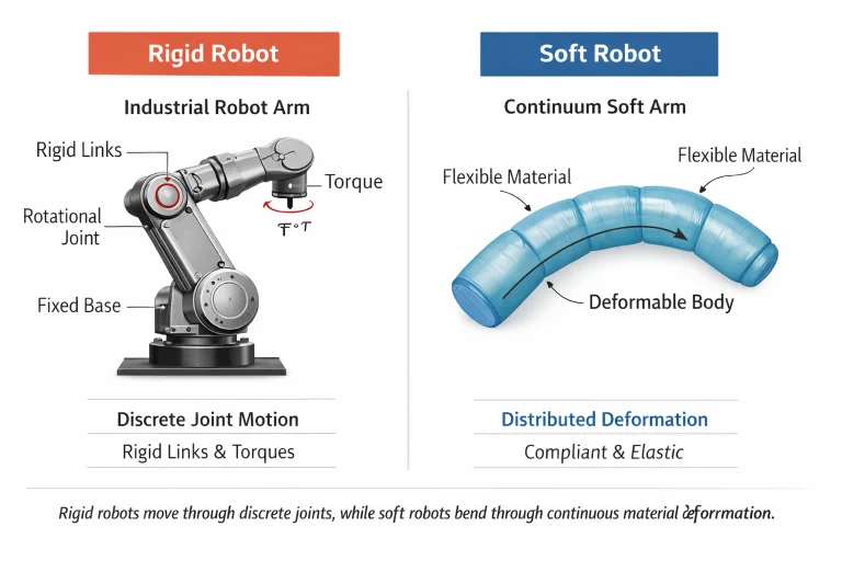
Kinematic comparison illustrating the transition from finite, discrete revolute joint coordinate vectors in rigid serial arms to infinite-dimensional continuum curves governed by continuous strain distributions.
Interactive Quick Review: Soft Robotics & Continuum Mechanics
Test your foundational understanding of distributed deformation versus rigid articulation before exploring continuum strain equations:
1. What is the fundamental difference in motion generation between rigid robots and soft robots?
2. What biological structures serve as the primary natural inspirations for continuum soft robotics?
Continuum Mechanics Foundations
Because soft robotic structures deform continuously, their motion cannot be modeled solely by standard Denavit-Hartenberg parameters or rigid body spatial transformations. Instead, engineers formulate kinematics and dynamics within the framework of continuum mechanics to describe continuous displacement, strain, and stress tensors.
Consider an infinitesimal elastomeric segment subjected to axial tension along its centerline:
- \(L\): original resting length
- \(\Delta L\): change in length after deformation
- \(F\): applied axial tensile force
- \(A\): cross-sectional area
The one-dimensional engineering strain \(\epsilon\) is defined as the fractional change in length:
$$ \epsilon = \frac{\Delta L}{L} $$The internal axial Cauchy stress \(\sigma\) represents the internal force distribution per unit area:
$$ \sigma = \frac{F}{A} $$For infinitesimal strains within the linear elastic regime, stress and strain obey Hooke’s law:
$$ \sigma = E \epsilon $$where \(E\) is Young’s modulus of elasticity. While structural metals (steel, titanium) exhibit moduli on the order of \(E \approx 10^{11} \text{ Pa}\), silicone polymers and hydrogels used in soft robotics range from \(E \approx 10^4 \text{ Pa}\) to \(10^6 \text{ Pa}\). This low elastic modulus enables high reversible strain capacity without plastic failure.
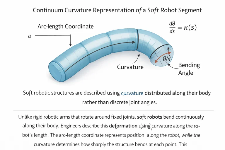
Differential geometric parameterization of a continuum segment: mapping the reference arc-length coordinate \(s\) to spatial curvature \(\kappa(s)\) and tangent orientation angle \(\theta(s)\).
Nonlinear and Hyperelastic Material Models
Soft robotic elastomers routinely undergo large finite deformations exceeding strains of \(100\%\) to \(500\%\). Under these non-infinitesimal regimes, linear Hookean approximations fail completely. Engineers turn to hyperelastic material models formulated via strain energy density functions \(W\).
For an isotropic, incompressible hyperelastic solid, the strain energy function is parameterized by the strain invariants \(I_1, I_2, I_3\) of the right Cauchy-Green deformation tensor \(\mathbf{C} = \mathbf{F}^T \mathbf{F}\), where \(\mathbf{F}\) is the deformation gradient:
$$ I_1 = \text{tr}(\mathbf{C}), \quad I_2 = \frac{1}{2}\left[(\text{tr}(\mathbf{C}))^2 - \text{tr}(\mathbf{C}^2)\right], \quad I_3 = \det(\mathbf{C}) = 1 \quad (\text{incompressible}) $$A standard formulation used for silicone matrices is the two-parameter Mooney–Rivlin model:
$$ W = C_1 (I_1 - 3) + C_2 (I_2 - 3) $$where \(C_1\) and \(C_2\) represent empirically measured material constants. For simpler low-strain approximations, setting \(C_2 = 0\) reduces the formulation to the neo-Hookean solid:
$$ W = C_1 (I_1 - 3) = \frac{\mu}{2}(I_1 - 3) $$where \(\mu\) is the initial shear modulus of the unpressurized elastomer.
Distributed Kinematics: The Piecewise Constant Curvature (PCC) Model
Rather than tracking a vector of discrete revolute joint angles \(\mathbf{q} = [q_1, q_2, \dots, q_n]^T\), a soft continuum segment is parameterized continuously over its curvilinear arc-length coordinate \(s \in [0, L]\).
Let \(\kappa(s)\) denote the continuous spatial curvature and \(\theta(s)\) the planar orientation angle along the backbone:
$$ \frac{d\theta(s)}{ds} = \kappa(s) \quad \Rightarrow \quad \theta(s) = \int_0^s \kappa(\xi) \, d\xi $$Under the Piecewise Constant Curvature (PCC) assumption, curvature is treated as spatially invariant along an isolated actuation section (\(\kappa(s) \equiv \kappa\)). For a segment of resting length \(L\), the total bending angle \(\theta\), radius of curvature \(R\), and spatial tip coordinates \((x, y)\) in the segment base frame evaluate to:
$$ R = \frac{1}{\kappa}, \quad \theta = \kappa L, \quad x = R(1 - \cos\theta) = \frac{1 - \cos(\kappa L)}{\kappa}, \quad y = R\sin\theta = \frac{\sin(\kappa L)}{\kappa} $$Actuation Mechanisms
Lacking conventional rigid gearboxes and high-torque rotary motors, soft robots embed distributed active functional materials into their structural skins.
- Pneumatic Networks (Pneu-Nets): Pressurizing asymmetrical embedded elastomer chambers induces differential longitudinal strain across opposing faces, forcing the structure to bend.
- Dielectric Elastomer Actuators (DEAs): High electric potentials (kilovolt scale) applied across compliant compliant electrodes squeeze a thin elastomer membrane via Maxwell stress, causing planar area expansion.
- Shape Memory Alloys (SMAs): Thermally activated crystalline phase changes (martensite to austenite) contract embedded Nitinol wires, functioning as artificial tendons.
- Fluidic Elastomer Actuators (FEAs): Pressurized hydraulic fluids provide higher working pressures and structural stiffness compared to compressible pneumatic channels.
For a pneumatic chamber of cross-sectional area \(A_c\) supplied with internal gauge pressure \(P\), the primary axial actuation force generated is approximated by:
$$ F_{\text{act}} = P A_c $$When this force acts at an eccentricity \(d\) from the neutral bending axis, it generates an internal bending moment \(M = F_{\text{act}} \cdot d = P A_c d\), driving continuum curvature.
Bio-Inspired Undulatory Locomotion
Soft crawling and swimming robots eliminate wheels and rigid tracks by reproducing continuous traveling deformation waves observed in anguilliform swimmers (eels, fish) and serpentine locomotion (snakes).
Planar traveling wave undulation can be modeled as a continuous harmonic function of arc-coordinate \(x\) and time \(t\):
$$ y(x, t) = A(x) \sin(kx - \omega t + \phi) $$where:
- \(A(x)\): position-dependent wave amplitude (frequently increasing toward the trailing edge)
- \(k = \frac{2\pi}{\lambda}\): spatial wavenumber (\(\text{rad}\cdot\text{m}^{-1}\)) with wavelength \(\lambda\)
- \(\omega = 2\pi f\): temporal angular frequency (\(\text{rad}\cdot\text{s}^{-1}\)) with frequency \(f\)
- \(\phi\): initial phase offset
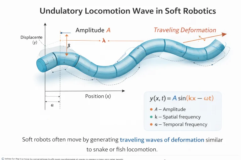
Kinematic wave parameterization tracking lateral displacement envelopes and spatial wavelength across elastomeric continuous bodies during fluidic or granular propulsion.
Adaptive Passive Grasping
A principal advantage of soft robotic manipulators is mechanical intelligence: delegating control complexity from closed-loop software algorithms into the physical compliance of the hardware.
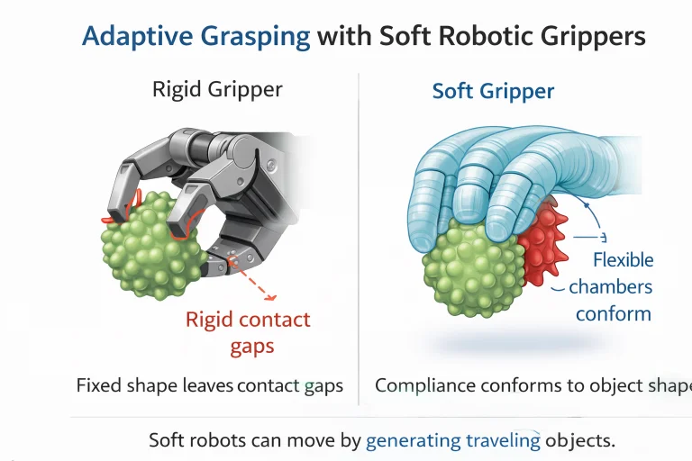
Morphological adaptation in multi-chambered elastomeric fingers: passive enveloping of complex, fragile surface geometries without tactile feedback matrices.
Human–Robot Interaction and Safety Compliance
In physical human-robot collaboration, safety is governed by peak kinetic impact forces and contact pressures. Industrial rigid arms possess high effective structural stiffness \(k_{\text{rigid}}\) and high reflected inertia, causing severe peak force spikes during accidental collision.
Modeling the contact interface as a linear elastic interaction over contact indentation depth \(\delta\):
$$ F_{\text{contact}} = k_{\text{eff}} \delta $$Because soft robots possess intrinsically compliant matrices (\(k_{\text{soft}} \ll k_{\text{rigid}}\)), the peak contact force generated during unexpected human contact remains strictly bounded well below tissue trauma thresholds, fulfilling intrinsic ISO/TS 15066 safety criteria without relying exclusively on sensor-triggered emergency stops.
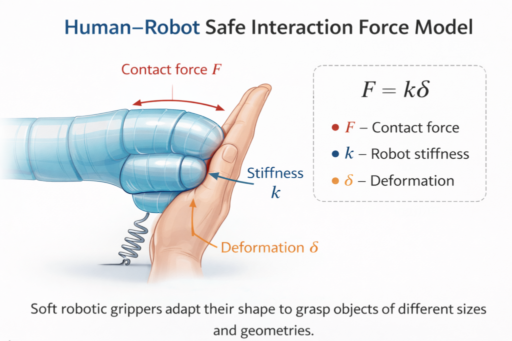
Biomechanical force attenuation model demonstrating how structural compliance absorbs kinetic energy and minimizes localized peak contact pressures during human interaction.
Contemporary 2026 Computational Paradigms: PINNs & Neural Operators
Classical continuum mechanics modeling faces severe limitations in real-time embedded control: solving nonlinear Cosserat rod equations or 3D hyperelastic finite element method (FEM) meshes requires millions of floating-point operations per time-step. To overcome this computational bottleneck, modern robotics combines analytical mechanics with deep learning frameworks.
1. Physics-Informed Neural Networks (PINNs)
Rather than treating soft deformation as an unconstrained black-box regression, PINNs embed the governing partial differential equations (PDEs) of continuum mechanics directly into the loss function. The residual of the momentum balance equation acts as a physical regularizer:
$$ \mathcal{L}_{\text{total}} = \mathcal{L}_{\text{data}} + \lambda_{\text{pde}} \mathcal{L}_{\text{pde}}, \quad \text{where} \quad \mathcal{L}_{\text{pde}} = \left\| \nabla \cdot \boldsymbol{\sigma} + \mathbf{b} - \rho \ddot{\mathbf{u}} \right\|^2 $$This architecture enables accurate internal stress and shape estimation from sparse surface-embedded strain sensors.
2. Fourier Neural Operators (FNOs) & DeepONets
In high-speed dynamic control, Fourier Neural Operators (FNOs) learn mappings between infinite-dimensional function spaces (e.g., mapping continuous chamber pressure distributions \(P(s, t)\) directly to time-resolved deformation fields \(\mathbf{u}(s, t)\)). By operating in the frequency domain via Fast Fourier Transforms (FFT), FNOs evaluate non-linear continuum dynamics orders of magnitude faster than numerical FEM solvers, enabling real-time Model Predictive Control (MPC) on microcontrollers.
History, Challenges, and Emerging Paradigms
Evolutionary Trajectory
Emerging from early 2000s biomimetics, soft robotics formalized into an autonomous discipline in the 2010s through the invention of multi-material 3D printing and lithography-molded fluidic networks (Pneu-Nets). Research has shifted from proof-of-concept passive elastomeric grippers to untethered autonomous bio-hybrid robots.
Current Engineering Bottlenecks
- Hysteresis & Viscoelastic Stress Relaxation: Elastomer chains dissipate mechanical energy internally, causing actuation strain to lag behind input pressure and drifting zero-state calibrations over cyclic loading.
- Infinite-Dimensional State Estimation: Lacking discrete pivot joints with rotary optical encoders, soft robots require stretchable liquid-metal (EGaIn) strain gauges or fiber Bragg gratings (FBG) to reconstruct spatial configuration.
- Payload vs. Compliance Trade-off: High elasticity inherently compromises load-carrying capacity; unsupported soft arms buckle under substantial lateral shear loads.
- Tethered Power Dependencies: Bulky off-board fluid pumps and compressors continue to hinder fully untethered field autonomy.
Interactive Quick Review: Hyperelasticity, Actuation & Neural Solvers
Verify your understanding of hyperelastic models, actuation mechanics, and modern data-driven continuum formulations before exploring the FAQ:
1. Why are hyperelastic strain energy functions (like Mooney-Rivlin) mandatory for elastomer modeling?
2. How do Fourier Neural Operators (FNOs) resolve the real-time control bottleneck of soft robots?
External References and Further Reading
Consult the following peer-reviewed academic literature and research repositories for deeper study:
- Nature Reviews Materials – Soft Robotics Focus – Authoritative treatises covering hyperelastic materials, bio-hybrid actuators, and electro-active polymers.
- Wyss Institute at Harvard University – Soft Robotics Lab – Open-source toolkits for pneumatic networks (Pneu-Nets) and autonomous soft machine architectures.
- Soft Robotics Journal (Liebertpub) – The primary international journal reporting advances in continuum mechanics, proprioceptive artificial skins, and biomimetic locomotion.
Frequently Asked Questions about Soft Robotics and Bio-Inspired Systems
What are the primary advantages of soft robots over traditional rigid industrial arms?
Soft robots provide intrinsic mechanical compliance, collision safety (\(F = k\delta\)), passive envelope grasping of delicate geometries, and environmental adaptability without complex high-bandwidth closed-loop force sensing.
How do pneumatic networks (Pneu-Nets) produce bending without discrete mechanical hinges?
Pneu-Nets bond an expandable elastomeric layer containing molded micro-channels to a strain-limiting, inextensible backing layer. Internal pressurization causes the expansion layer to elongate while the base layer maintains fixed length, forcing the entire composite beam to bend into an arc.
Why is state estimation difficult in continuous soft robotic structures?
Unlike rigid arms defined by finite joint coordinate vectors \(\mathbf{q} \in \mathbb{R}^n\), continuum structures exhibit theoretically infinite degrees of freedom. Reconstructing shape requires distributed sensory arrays (e.g., optical fibers, liquid metal resistance sensors) combined with PDE-based state observers or neural surrogates.
What is the Piecewise Constant Curvature (PCC) assumption in continuum mechanics?
The PCC approximation assumes that individual sections of a soft manipulator bend uniformly into circular arcs with constant curvature \(\kappa(s) \equiv \kappa\). This dramatically simplifies kinematic calculations by replacing partial differential equations with closed-form geometric transformations.
How does mechanical compliance protect humans during physical collaboration?
Low effective structural stiffness \(k_{\text{eff}}\) ensures that collision energy is dissipated through material deformation (\(\delta\)) rather than high impulse shocks. As expressed by \(F = k_{\text{eff}} \delta\), minimizing stiffness bounds contact forces below injury thresholds.
What are shape memory alloys (SMAs), and how do they actuate soft robots?
SMAs (such as nickel-titanium Nitinol) undergo a crystalline phase transition between low-temperature martensite and high-temperature austenite when heated via Joule heating. This transition produces substantial axial contraction forces (often exceeding \(200 \text{ MPa}\)), acting as compact artificial muscles.
Why do soft robots have lower payload capacities than rigid metallic arms?
Low material elastic moduli make compliant manipulators vulnerable to gravitational sagging, torsional twisting, and structural buckling under heavy cantilevered loads. Increasing payload capacity requires variable-stiffness mechanisms like granular jamming or tendon stiffening.
What professional career specializations exist in soft robotics?
Key career tracks include soft actuator design, biomimetic systems engineering, medical wearable robotics, smart prosthetics development, computational material modeling, and agricultural handling automation.
End-of-Page Exercises: Review, Conceptual Analysis & Derivations
Part I: Review Questions
1. How is engineering strain \(\epsilon\) defined for a deforming elastomer segment?
2. State Hooke’s law relating axial stress \(\sigma\) to strain \(\epsilon\) for small linear elastic deformations.
3. What equation expresses the strain energy density \(W\) in the two-parameter Mooney–Rivlin model?
4. How does local curvature \(\kappa(s)\) relate to tangent angle \(\theta(s)\) along arc length \(s\)?
5. Write the equation approximating pneumatic actuation force \(F\) from internal chamber pressure \(P\) and cross-sectional area \(A_c\).
6. State the traveling harmonic wave equation modeling bio-inspired undulatory locomotion.
7. How does contact force \(F\) relate to structural compliance stiffness \(k\) and indentation deformation \(\delta\)?
8. List four key operational advantages of soft robots compared to rigid serial link arms.
9. What mechanical property allows soft grippers to secure unknown objects without tactile feedback?
10. Name five engineering and mathematical disciplines foundational to soft robotics research.
Part II: Thought-Provoking Conceptual Questions
1. Why does continuous deformation produce an infinite-dimensional configuration space, and how does this challenge feedback control?
2. How does viscoelastic hysteresis in silicone elastomers cause actuation lag and positional drift during cyclic loading?
3. What are the engineering trade-offs when transitioning from tethered compressors to onboard catalytic gas generation?
4. How do coupled Fluid-Structure Interaction (FSI) phenomena affect underwater biomimetic soft fins?
5. Why is proprioception (internal state sensing) difficult to implement in high-strain elastomeric actuators?
6. In what way does morphological compliance substitute for digital algorithmic control in soft grasping?
7. How does elastic buckling instability transform from a structural failure mode into a rapid actuation mechanism in soft machines?
8. What microfabrication and physics barriers emerge when scaling soft actuators down to sub-millimeter scales for endovascular surgery?
9. How do scientific machine learning methods (such as PINNs and Neural Operators) bypass traditional finite element limitations in real-time control?
10. What micro-structural failure modes cause pneumatic elastomeric actuators to burst under cyclic pressure?
11. How does intentional fiber-reinforcement anisotropy direct multi-degree-of-freedom deformation in soft actuators?
12. Why do bio-inspired peristaltic earthworm robots navigate tight underground conduits more effectively than wheeled rovers?
Part III: Step-by-Step Numerical Engineering Derivations
Problem 1: Engineering Strain Calculation for an Inflated Elastomer
Scenario: A soft robotic pneumatic actuator segment has an initial resting length \(L = 150.0 \text{ mm}\). When pressurized, the segment extends to a length of \(L_{\text{new}} = 210.0 \text{ mm}\). Calculate the length change \(\Delta L\) and determine the resulting engineering strain \(\epsilon\) as both a decimal and percentage.
Step-by-Step Derivation:
$$ \begin{aligned} \Delta L &= L_{\text{new}} - L = 210.0 \text{ mm} - 150.0 \text{ mm} = 60.0 \text{ mm} \\ \epsilon &= \frac{\Delta L}{L} = \frac{60.0 \text{ mm}}{150.0 \text{ mm}} = 0.40 \\ \epsilon_{\%} &= 0.40 \times 100\% = 40.0\% \end{aligned} $$Answer & Conclusion: The elongation is \(60.0 \text{ mm}\), producing an engineering strain of \(\epsilon = 0.40\) (\(40.0\%\) tensile elongation).
Problem 2: Linear Elastic Stress and Young’s Modulus Sizing
Scenario: A soft artificial muscle strip with cross-sectional area \(A = 1.2 \text{ cm}^2\) (\(1.2 \times 10^{-4} \text{ m}^2\)) experiences an axial pulling force \(F = 18.0 \text{ N}\). The measured axial strain is \(\epsilon = 0.05\) (\(5.0\%\)). Compute the internal axial stress \(\sigma\) in Pascals and find Young’s modulus \(E\) in kilopascals (kPa).
Step-by-Step Derivation:
$$ \begin{aligned} \sigma &= \frac{F}{A} = \frac{18.0 \text{ N}}{1.2 \times 10^{-4} \text{ m}^2} = 150{,}000 \text{ Pa} = 150.0 \text{ kPa} \\ E &= \frac{\sigma}{\epsilon} = \frac{150{,}000 \text{ Pa}}{0.05} = 3{,}000{,}000 \text{ Pa} = 3{,}000 \text{ kPa} \quad (3.0 \text{ MPa}) \end{aligned} $$Answer & Conclusion: The internal stress is \(\sigma = 150.0 \text{ kPa}\) and the calculated elastic modulus is \(E = 3{,}000 \text{ kPa}\) (\(3.0 \text{ MPa}\)), consistent with soft polyurethane or silicone rubbers.
Problem 3: Mooney–Rivlin Hyperelastic Strain Energy Density
Scenario: An elastomeric finger joint wall is modeled via the Mooney–Rivlin strain energy function \(W = C_1(I_1 - 3) + C_2(I_2 - 3)\). Empirical characterization yields \(C_1 = 120.0 \text{ kPa}\) and \(C_2 = 25.0 \text{ kPa}\). During an inflation step, deformation invariants are computed as \(I_1 = 4.2\) and \(I_2 = 3.8\). Calculate the stored strain energy density \(W\).
Step-by-Step Derivation:
$$ \begin{aligned} I_1 - 3 &= 4.2 - 3.0 = 1.2 \\ I_2 - 3 &= 3.8 - 3.0 = 0.8 \\ W_1 &= C_1 (I_1 - 3) = 120.0 \text{ kPa} \times 1.2 = 144.0 \text{ kPa} \\ W_2 &= C_2 (I_2 - 3) = 25.0 \text{ kPa} \times 0.8 = 20.0 \text{ kPa} \\ W &= W_1 + W_2 = 144.0 \text{ kPa} + 20.0 \text{ kPa} = 164.0 \text{ kPa} \end{aligned} $$Answer & Conclusion: The total hyperelastic strain energy density is \(W = 164.0 \text{ kPa}\) (\(1.64 \times 10^5 \text{ J}\cdot\text{m}^{-3}\)).
Problem 4: Actuation Force in a Pneumatic Expansion Chamber
Scenario: A cylindrical fluid chamber in a soft gripper has a diameter \(D = 2.0 \text{ cm}\) (radius \(r = 1.0 \text{ cm} = 0.01 \text{ m}\)). The supply regulator supplies an internal gauge pressure \(P = 120.0 \text{ kPa}\) (\(120{,}000 \text{ N}\cdot\text{m}^{-2}\)). Calculate the chamber cross-sectional area \(A_c\) and find the resulting actuation force \(F_{\text{act}}\).
Step-by-Step Derivation:
$$ \begin{aligned} A_c &= \pi r^2 = \pi \times (0.01 \text{ m})^2 = 3.14159 \times 10^{-4} \text{ m}^2 \\ F_{\text{act}} &= P A_c = 120{,}000 \text{ N}\cdot\text{m}^{-2} \times 3.14159 \times 10^{-4} \text{ m}^2 \approx 37.70 \text{ N} \end{aligned} $$Answer & Conclusion: The internal area is \(A_c \approx 3.142 \times 10^{-4} \text{ m}^2\), generating an axial actuation force of \(F_{\text{act}} \approx 37.70 \text{ N}\).
Problem 5: Constant Curvature Kinematic Bending Angle
Scenario: A continuum manipulator segment of arc length \(L = 0.30 \text{ m}\) deforms uniformly with constant curvature \(\kappa = 4.0 \text{ m}^{-1}\). Calculate the total tip bending angle \(\theta\) in radians and convert to degrees (using \(1 \text{ rad} \approx 57.2958^\circ\)).
Step-by-Step Derivation:
$$ \begin{aligned} \theta &= \kappa L = 4.0 \text{ m}^{-1} \times 0.30 \text{ m} = 1.20 \text{ radians} \\ \theta_{\text{deg}} &= 1.20 \text{ rad} \times 57.2958^\circ/\text{rad} \approx 68.75^\circ \end{aligned} $$Answer & Conclusion: The continuous bending angle across the segment is \(\theta = 1.20 \text{ rad}\) (\(68.75^\circ\)).
Problem 6: Kinematic Position of an Undulatory Traveling Wave
Scenario: A soft biomimetic swimmer follows the harmonic traveling wave profile \(y(x, t) = A \sin(kx - \omega t)\). Parameters are amplitude \(A = 0.08 \text{ m}\), spatial wavenumber \(k = 5.0 \text{ rad}\cdot\text{m}^{-1}\), and temporal frequency \(\omega = 10.0 \text{ rad}\cdot\text{s}^{-1}\). Calculate the lateral displacement \(y\) at position \(x = 0.5 \text{ m}\) and time \(t = 0.2 \text{ s}\).
Step-by-Step Derivation:
$$ \begin{aligned} \text{Phase } \Phi &= kx - \omega t = (5.0 \times 0.5) - (10.0 \times 0.2) = 2.5 - 2.0 = 0.5 \text{ rad} \\ \sin(0.5 \text{ rad}) &\approx 0.479426 \\ y(0.5, 0.2) &= 0.08 \text{ m} \times 0.479426 \approx 0.03835 \text{ m} \quad (3.84 \text{ cm}) \end{aligned} $$Answer & Conclusion: At \(x = 0.5 \text{ m}\) and \(t = 0.2 \text{ s}\), the lateral displacement is \(y \approx 0.0384 \text{ m}\) (\(3.84 \text{ cm}\)).
Problem 7: Human–Robot Impact Force Attenuation
Scenario: An assistive soft exoskeleton joint exhibits effective stiffness \(k = 2{,}500.0 \text{ N}\cdot\text{m}^{-1}\). During accidental collision with a human limb, the joint deforms by \(\delta = 12.0 \text{ mm}\) (\(0.012 \text{ m}\)). Calculate the resulting contact force \(F_{\text{contact}}\) and compare it against an unyielding rigid robot arm producing \(F_{\text{rigid}} = 250.0 \text{ N}\).
Step-by-Step Derivation:
$$ \begin{aligned} F_{\text{contact}} &= k \delta = 2{,}500.0 \text{ N}\cdot\text{m}^{-1} \times 0.012 \text{ m} = 30.0 \text{ N} \\ \text{Force Reduction Ratio} &= \frac{F_{\text{rigid}} - F_{\text{contact}}}{F_{\text{rigid}}} = \frac{250.0 - 30.0}{250.0} = \frac{220.0}{250.0} = 0.88 \quad (88.0\%) \end{aligned} $$Answer & Conclusion: The compliant contact force is \(F = 30.0 \text{ N}\), achieving an \(88.0\%\) reduction in peak force compared to the rigid system.
Problem 8: Radius of Curvature for a Continuum Catheter
Scenario: A soft medical steering catheter bends into a circular arc with measured curvature \(\kappa = 5.0 \text{ m}^{-1}\). Calculate the radius of curvature \(R\) in meters and centimeters.
Step-by-Step Derivation:
$$ \begin{aligned} R &= \frac{1}{\kappa} = \frac{1}{5.0 \text{ m}^{-1}} = 0.20 \text{ m} \\ R_{\text{cm}} &= 0.20 \text{ m} \times 100 \text{ cm}\cdot\text{m}^{-1} = 20.0 \text{ cm} \end{aligned} $$Answer & Conclusion: The radius of curvature is \(R = 0.20 \text{ m}\) (\(20.0 \text{ cm}\)).
Problem 9: Elastomer Component Volume and Mass Sizing
Scenario: A soft silicone actuator slab has dimensions of length \(L = 0.20 \text{ m}\), width \(w = 0.05 \text{ m}\), and thickness \(t = 0.01 \text{ m}\). The density of the cross-linked polymer is \(\rho = 1{,}100.0 \text{ kg}\cdot\text{m}^{-3}\). Calculate total volume \(V\) and total mass \(M\) in grams.
Step-by-Step Derivation:
$$ \begin{aligned} V &= L \times w \times t = 0.20 \text{ m} \times 0.05 \text{ m} \times 0.01 \text{ m} = 0.00010 \text{ m}^3 = 1.0 \times 10^{-4} \text{ m}^3 \\ M &= \rho V = 1{,}100.0 \text{ kg}\cdot\text{m}^{-3} \times 1.0 \times 10^{-4} \text{ m}^3 = 0.110 \text{ kg} \\ M_{\text{grams}} &= 0.110 \text{ kg} \times 1{,}000 \text{ g}\cdot\text{kg}^{-1} = 110.0 \text{ g} \end{aligned} $$Answer & Conclusion: The slab volume is \(1.0 \times 10^{-4} \text{ m}^3\), with a total structural mass of \(M = 110.0 \text{ g}\).
Problem 10: Shape Memory Alloy (SMA) Micro-Wire Pulling Force
Scenario: A Nitinol shape memory alloy wire embedded in a soft finger has diameter \(d = 0.50 \text{ mm}\) (radius \(r = 0.25 \text{ mm} = 2.5 \times 10^{-4} \text{ m}\)). Upon electrical heating, the alloy undergoes a phase transformation that generates an axial contraction stress \(\sigma_{\text{sma}} = 200.0 \text{ MPa}\) (\(2.0 \times 10^8 \text{ N}\cdot\text{m}^{-2}\)). Compute cross-sectional area \(A\) and the resulting contraction force \(F_{\text{sma}}\).
Step-by-Step Derivation:
$$ \begin{aligned} A &= \pi r^2 = \pi \times (2.5 \times 10^{-4} \text{ m})^2 \approx 1.9635 \times 10^{-7} \text{ m}^2 \\ F_{\text{sma}} &= \sigma_{\text{sma}} A = (2.0 \times 10^8 \text{ N}\cdot\text{m}^{-2}) \times (1.9635 \times 10^{-7} \text{ m}^2) \approx 39.27 \text{ N} \end{aligned} $$Answer & Conclusion: The wire cross-section is \(A \approx 1.964 \times 10^{-7} \text{ m}^2\), generating a pulling force of \(F_{\text{sma}} \approx 39.27 \text{ N}\).
Problem 11: Viscoelastic Stress Relaxation Force Decay
Scenario: A soft elastomer gripper finger exerts an instantaneous peak holding force \(F_0 = 50.0 \text{ N}\) upon closing. Viscoelastic relaxation causes the force to decay according to \(F(t) = F_0 e^{-t/\tau}\), where the relaxation time constant is \(\tau = 15.0 \text{ s}\). Calculate the remaining holding force after \(t = 30.0 \text{ s}\) (using \(e^{-2.0} \approx 0.135335\)).
Step-by-Step Derivation:
$$ \begin{aligned} \frac{t}{\tau} &= \frac{30.0 \text{ s}}{15.0 \text{ s}} = 2.0 \\ F(30.0) &= F_0 e^{-2.0} = 50.0 \text{ N} \times 0.135335 \approx 6.77 \text{ N} \end{aligned} $$Answer & Conclusion: Viscoelastic stress relaxation reduces the holding force to \(F(30) \approx 6.77 \text{ N}\) over 30 seconds.
Problem 12: Fluid Expansion Volumetric Strain Ratio
Scenario: A pneumatic chamber in an elastomeric actuator has an initial unpressurized volume \(V_0 = 15.0 \text{ cm}^3\). Upon full pressurization, the chamber inflates to an expanded volume \(V_{\text{final}} = 37.5 \text{ cm}^3\). Compute the volumetric difference \(\Delta V\) and determine the volumetric expansion ratio \(V_{\text{final}} / V_0\).
Step-by-Step Derivation:
$$ \begin{aligned} \Delta V &= V_{\text{final}} - V_0 = 37.5 \text{ cm}^3 - 15.0 \text{ cm}^3 = 22.5 \text{ cm}^3 \\ \text{Expansion Ratio} &= \frac{V_{\text{final}}}{V_0} = \frac{37.5 \text{ cm}^3}{15.0 \text{ cm}^3} = 2.50 \end{aligned} $$Answer & Conclusion: The internal chamber volume expands by \(22.5 \text{ cm}^3\), representing a \(2.50\times\) expansion ratio.
Soft Robotics and Bio-Inspired Systems — Summary & Wrap-Up
Soft robotics bridges the gap between synthetic machines and living organisms by replacing rigid components with compliant materials. Grounded in continuum mechanics and hyperelastic material formulations (such as the Mooney–Rivlin model), soft systems distribute deformation along continuous curves rather than discrete pivot joints. Pneumatic network actuation, fiber reinforcement, and undulatory kinematic profiles allow these robots to achieve delicate grasping, safe human-robot collaboration, and locomotion in tortuous environments.
Looking forward, modern computational tools—such as Physics-Informed Neural Networks (PINNs) and Fourier Neural Operators (FNOs)—bypass traditional finite element bottlenecks to make real-time closed-loop control of infinite-degree-of-freedom continuum machines practical.