
Robotic digital twin systems extend the concept of virtual simulation directly into live, operational execution. Rather than modeling an autonomous system solely during early architectural design or isolated pre-deployment phases, a robotic digital twin maintains a continuously synchronized virtual replica of a physical robot while that robot actively operates in the real world.
Unlike traditional static simulation models that run offline, a robotic digital twin evolves dynamically as the physical machine navigates, acquires sensory measurements, and interacts with unstructured environments. Real-time joint telemetry, control inputs, and environmental states are streamed from the physical robot to its digital counterpart. This bidirectional pipeline allows engineers to monitor operational behavior, predict mechanical failures, and evaluate experimental control policies in parallel with real-world execution.
Robotic digital twins form an integral part of the broader robotics software infrastructure, functioning alongside high-fidelity simulation platforms, middleware communication layers, embedded controllers, and distributed edge computing clusters. Together, these technologies enable robots to be tested, optimized, and maintained across interconnected physical and virtual domains.
Whereas broader industrial digital twins model facility-wide manufacturing lines or regional logistics infrastructure, robotic digital twins focus specifically on the multi-body physics, sensor perception, real-time control, and adaptive intelligence of an individual robotic platform. For large-scale manufacturing plant modeling, explore Digital Twin Technology.
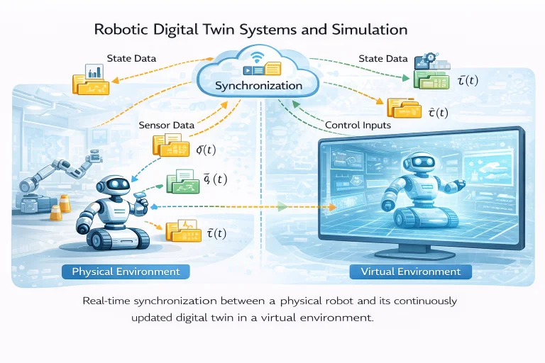
This architecture illustrates the continuous synchronization cycle connecting physical robots with virtual simulation twins. The operating hardware streams measured joint positions, velocities, motor currents, and perception feeds over deterministic network buses to the digital twin. The virtual replica updates its internal numerical dynamics and state estimators to mirror physical behavior. Concurrently, the digital twin executes predictive safety simulations, synthetic sensor generation, and anomaly detection algorithms, feeding optimized trajectory waypoints or safety stops back to the physical platform.
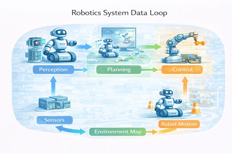
Interactive Quick Review: Real-Time Twins & Synchronization
Test your understanding of digital twin state mirroring versus offline simulation before exploring state synchronization equations:
1. What is the fundamental operational difference between a traditional offline robot simulation and a robotic digital twin?
Answer: Traditional simulations execute offline in isolation using pre-programmed parameters prior to deployment. A robotic digital twin maintains a continuous, live, bidirectional telemetry pipeline with an active physical robot during live operation, updating internal state variables in real time.
2. How does real-time physical telemetry improve the accuracy of the virtual simulation model over time?
Answer: Real-world sensor observations (joint angles, torque loads, thermal changes) continuously correct internal state estimators and update dynamic model parameters, preventing integration drift and tuning the simulator to match physical reality.
Glossary of Key Terminology
Essential mathematical, architectural, and simulation terms governing robotic digital twins, Hardware-in-the-Loop environments, and state synchronization:
State Synchronization Between Physical and Virtual Systems
A robotic digital twin continuously mirrors the internal kinematic and dynamic state vectors of the physical machine. Let the physical state vector at continuous time \(t\) be defined as:
$$\mathbf{x}(t) = \begin{bmatrix} \mathbf{q}(t) \\ \dot{\mathbf{q}}(t) \\ \boldsymbol{\tau}(t) \end{bmatrix} \in \mathbb{R}^{3n}$$where \(\mathbf{q}(t) \in \mathbb{R}^n\) denotes generalized joint coordinates, \(\dot{\mathbf{q}}(t) \in \mathbb{R}^n\) represents joint velocities, and \(\boldsymbol{\tau}(t) \in \mathbb{R}^n\) represents active actuator torques across \(n\) degrees of freedom.
The digital twin maintains internal estimated state vectors:
$$\hat{\mathbf{x}}(t) = \begin{bmatrix} \hat{\mathbf{q}}(t) \\ \hat{\dot{\mathbf{q}}}(t) \\ \hat{\boldsymbol{\tau}}(t) \end{bmatrix}$$True synchronization requires bounding the tracking error norm across operational intervals:
$$\|\mathbf{q}(t) - \hat{\mathbf{q}}(t)\| \le \epsilon_{\text{sync}}, \quad \forall t \ge 0$$Discrepancies between physical states and virtual estimates arise from unmodeled physical dynamics (e.g., thermal expansions, cable compliance), stochastic sensor noise, and network communication latency.
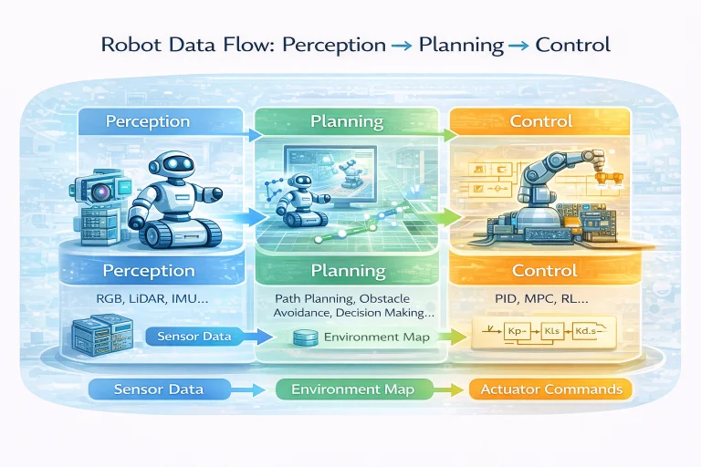
Dynamic Modeling & Numerical Physics Integration
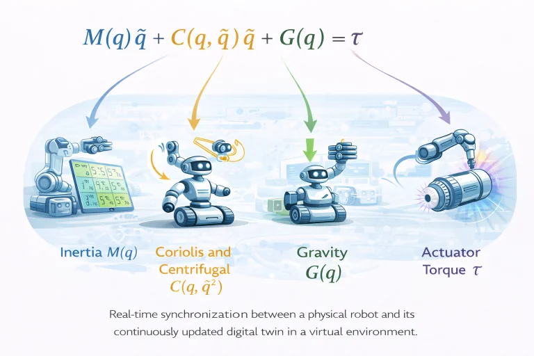
The physics engine inside a robotic digital twin simulates continuous rigid-body mechanics by integrating the non-linear multi-body equations of motion:
$$\mathbf{M}(\mathbf{q})\ddot{\mathbf{q}} + \mathbf{C}(\mathbf{q}, \dot{\mathbf{q}})\dot{\mathbf{q}} + \mathbf{G}(\mathbf{q}) + \mathbf{F}_{\text{ext}}(\mathbf{q}, \dot{\mathbf{q}}) = \boldsymbol{\tau}$$where:
- \(\mathbf{M}(\mathbf{q}) \in \mathbb{R}^{n \times n}\): Symmetric, positive-definite Generalized Inertia Matrix.
- \(\mathbf{C}(\mathbf{q}, \dot{\mathbf{q}})\dot{\mathbf{q}} \in \mathbb{R}^n\): Coriolis and centrifugal torque vector.
- \(\mathbf{G}(\mathbf{q}) \in \mathbb{R}^n\): Gravitational torque vector derived from potential energy gradients.
- \(\mathbf{F}_{\text{ext}} \in \mathbb{R}^n\): External environmental interaction forces (contact constraints, Coulomb and viscous friction).
- \(\boldsymbol{\tau} \in \mathbb{R}^n\): Vector of commanded actuator joint torques.
To advance the simulation in discrete virtual time, the physics engine solves for instantaneous joint accelerations:
$$\ddot{\mathbf{q}} = \mathbf{M}^{-1}(\mathbf{q}) \left[ \boldsymbol{\tau} - \mathbf{C}(\mathbf{q}, \dot{\mathbf{q}})\dot{\mathbf{q}} - \mathbf{G}(\mathbf{q}) - \mathbf{F}_{\text{ext}} \right]$$Numerical integration techniques (such as semi-implicit Euler or Fourth-Order Runge-Kutta) advance velocities and positions across discrete simulation time steps \(h\):
$$\dot{\mathbf{q}}_{k+1} = \dot{\mathbf{q}}_k + h \ddot{\mathbf{q}}_k, \quad \mathbf{q}_{k+1} = \mathbf{q}_k + h \dot{\mathbf{q}}_{k+1}$$Hardware-in-the-Loop (HIL) Architecture
Hardware-in-the-Loop (HIL) simulation splits execution across physical hardware and virtual simulation. Embedded controllers (e.g., motor drive DSPs, flight microcontrollers) execute production firmware, while the mechanical plant, environmental sensors, and external dynamics are computed in real time by the digital twin platform.

The closed-loop timing cycle must satisfy hard real-time latency bounds:
$$\mathbf{u}_{\text{hardware}}(t) \Rightarrow{\text{Bus Interface}} \text{Digital Twin (Physics)} \Rightarrow{\text{Sensor Emulation}} \mathbf{y}_{\text{sensor}}(t) \Rightarrow{\text{Bus Interface}} \text{Hardware Controller}$$If round-trip transport delay \(\tau_d\) exceeds a fraction of the digital control loop sampling period \(T_s\) (typically \(\tau_d / T_s > 0.10\)), unmodeled transport lag degrades the open-loop phase margin \(\Phi_m\), inducing control chatter or closed-loop instability.
Engineering Challenges & Technical Solutions
Building real-time, high-fidelity robotic digital twins introduces several practical electromechanical, algorithmic, and networking challenges:
The Challenge: Streaming raw sensor data across standard wireless networks (Wi-Fi, 5G) introduces non-deterministic packet jitter and multi-millisecond latency. If a digital twin attempts direct closed-loop feedback control, transport delay induces phase lag that can destabilize high-speed robot joints.
- Hierarchical Control Partitioning: Restricting the digital twin to supervisory setpoint optimization and predictive diagnostics, while delegating high-frequency (1 kHz) closed-loop stabilization to local embedded microcontrollers, as outlined in Real-Time Embedded Systems in Robotics.
- Predictive State Observers & Kalman Filtering: Using Extended Kalman Filters (EKF) inside the digital twin to forward-propagate dynamic models during communication dropouts, bridging latency gaps.
The Challenge: Rigid-body physics engines model physical contacts (e.g., robotic fingers grasping an object or quadruped foot impacts) using hard non-penetration constraints. Discontinuous contact force switching causes numerical instability, penetration artifacts, and solver divergence.
- Linear Complementarity Problem (LCP) Solvers: Formulating contact constraints via projected Gauss-Seidel or Dantzig algorithms to solve multi-point friction cones simultaneously.
- Compliant Contact Modeling: Utilizing regularized spring-damper contact models (e.g., Hunt-Crossley model) that smooth force transitions over small penetrations, preserving numerical stability.
The Challenge: Control policies trained purely in virtual simulation often fail when deployed on physical robots due to unmodeled motor backlash, cable elasticity, micro-friction variations, and camera lens distortions.
- Domain Randomization: Randomly perturbing simulation dynamics (\(\mathbf{M} \to \mathbf{M} + \Delta \mathbf{M}\), friction, latency) during training, forcing policies to develop robustness across physical parameter variations.
- System Identification & Real2Sim Calibration: Running automated physical calibration routines to log joint trajectories, using non-linear least squares to update inertial parameters and friction curves in the simulation model.
The Challenge: In autonomous warehouse facilities housing hundreds of mobile robots, streaming continuous raw video feeds and point clouds to cloud digital twins can saturate industrial Wi-Fi networks.
- Edge Feature Extraction: Processing raw point clouds into lightweight obstacle bounding boxes and pose vectors onboard before transmitting telemetry to the central twin.
- Adaptive Telemetry QoS: Configuring ROS 2 DDS Quality of Service profiles to stream low-bandwidth state vectors continuously while throttling high-bandwidth image topics, as detailed in Robot Operating System (ROS and ROS 2).
Predictive Maintenance & Anomaly Detection
Digital twins continuously compare measured physical sensor signals against model-predicted baselines. For joint actuators, the scalar torque residual is defined as:
$$e_\tau(t) = \tau_{\text{meas}}(t) - \tau_{\text{pred}}(t)$$where \(\tau_{\text{meas}}(t)\) is derived from motor current measurements and \(\tau_{\text{pred}}(t)\) is computed via the inverse dynamics model (\(\mathbf{M}\ddot{\mathbf{q}} + \mathbf{C}\dot{\mathbf{q}} + \mathbf{G}\)).
Under healthy operating conditions, the residual represents mean-zero Gaussian sensor noise: \(\mathbb{E}[e_\tau(t)] \approx 0\). When mechanical degradation begins (e.g., bearing wear, lack of lubrication, or gear tooth pitting), friction torques rise, generating a persistent positive residual offset:
$$\int_{t_0}^{t_0 + T} e_\tau(t) \, dt > \gamma_{\text{threshold}}$$Early detection of these residual shifts enables automated predictive maintenance alerts before catastrophic mechanical failure occurs.
Interactive Quick Review: HIL, Domain Randomization & Anomaly Detection
Reinforce key concepts regarding Hardware-in-the-Loop architectures, residual torque monitoring, and sim-to-real policies before reviewing the FAQ:
1. How does torque residual tracking (\(e_\tau(t) = \tau_{\text{meas}}(t) - \tau_{\text{pred}}(t)\)) enable predictive maintenance in a digital twin?
Answer: By continuously subtracting model-predicted torques from physical motor sensor currents; a growing positive residual indicates unmodeled friction, bearing degradation, or gear wear before mechanical failure occurs.
2. What is the role of middleware frameworks (such as ROS 2 / DDS) in Hardware-in-the-Loop (HIL) testing?
Answer: Middleware provides low-latency, deterministic transport layers that stream real sensor inputs (\(y_{\text{sensor}}\)) into virtual simulation engines and route computed virtual control actions (\(u_{\text{sim}}\)) back to physical hardware.
External References and Further Reading
To explore physics engines, industrial digital twin architectures, and HIL simulation standards, consult the following authoritative sources:
- NVIDIA Isaac Sim & Omniverse – A physically accurate simulation platform for training AI control policies and conducting digital twin validations.
- Gazebo Physics Simulation Environment – An open-source 3D robotics simulator supporting ODE, Bullet, and DART physics engines integrated with ROS 2.
- Ansys Digital Twin Platform – Multiphysics modeling suite used to simulate thermal, structural, and electromagnetic dynamics in physical systems.
Frequently Asked Questions about Robotic Digital Twin Systems and Simulation
What is the difference between a 3D simulation model and a true Digital Twin?
A standard 3D simulation runs offline in isolation using pre-programmed parameters. A true Digital Twin maintains a continuous, live, two-way telemetry connection with an operating physical robot, updating state estimates (\(\hat{\mathbf{q}}(t) \approx \mathbf{q}(t)\)) and adapting dynamic parameters to mirror real-world changes continuously.
What is Hardware-in-the-Loop (HIL) simulation, and why is it used?
HIL simulation interfaces physical hardware components (such as an embedded ECU or motor drive) with a simulated physics environment. It permits testing control code and fault-recovery routines on real silicon under extreme simulated hazard conditions without risking physical robot destruction.
How does domain randomization bridge the "sim-to-real gap"?
Domain randomization injects random variations into simulated physical properties (e.g., link masses \(\mathbf{M} \to \mathbf{M} + \Delta \mathbf{M}\), friction coefficients, surface textures) during policy training. This forces reinforcement learning policies to discover generalized strategies that transfer reliably to physical hardware (\(\pi_{\text{real}} \approx \pi_{\text{sim}}\)).
How do digital twins enable predictive maintenance in automated factories?
The twin continuously evaluates residual error signals between physical measurements and virtual predictions (\(e_\tau(t) = \tau_{\text{meas}}(t) - \tau_{\text{pred}}(t)\)). A persistent, unexplained rise in residual error serves as an early indicator of bearing wear, backlash, or thermal degradation long before physical breakdown occurs.
What causes state synchronization latency in cloud-connected digital twins?
Synchronization latency stems from sensor sampling rates, network packet serialization, wireless propagation delays, and cloud data processing overhead. If latency \(\tau_d\) exceeds a significant fraction of the control period \(T_s\), state estimates lag, limiting cloud twins to supervisory monitoring rather than direct high-speed closed-loop control.
Which physics engines are commonly used to power robotic digital twins?
Widely used physics engines include PhysX (NVIDIA Isaac Sim), Bullet Physics, DART, and ODE (Gazebo). These engines use numerical integration schemes (like semi-implicit Euler or Runge-Kutta) to solve rigid-body dynamic equations \(\mathbf{M}(\mathbf{q})\ddot{\mathbf{q}} + \mathbf{C}(\mathbf{q}, \dot{\mathbf{q}})\dot{\mathbf{q}} + \mathbf{G}(\mathbf{q}) = \boldsymbol{\tau}\) in real time.
End-of-Page Exercises: Review, Thought-Provoking & Engineering Problems
Section 1: Foundational Review Questions & Answers
1. What condition defines accurate position state synchronization in a robotic digital twin?
Answer: \(\hat{\mathbf{q}}(t) \approx \mathbf{q}(t)\), indicating that the estimated twin joint configuration vector tracks the physical robot joint position vector in real time within bound \(\epsilon_{\text{sync}}\).
2. What fundamental equation governs dynamic torque computation in rigid-body robotic twins?
Answer: \(\mathbf{M}(\mathbf{q})\ddot{\mathbf{q}} + \mathbf{C}(\mathbf{q}, \dot{\mathbf{q}})\dot{\mathbf{q}} + \mathbf{G}(\mathbf{q}) = \boldsymbol{\tau}\).
3. What does \(\mathbf{M}(\mathbf{q})\) represent in the dynamic equation of a robot?
Answer: The configuration-dependent, symmetric, positive-definite mass and inertia matrix of the manipulator.
4. What signal flow loop characterizes a Hardware-in-the-Loop (HIL) simulation?
Answer: \(\mathbf{u}_{\text{sim}}(t) \to \text{hardware} \to \mathbf{y}_{\text{sensor}}(t)\), routing simulated control outputs to physical hardware and returning real sensor feedback into the simulation platform.
5. How is relative HIL communication delay evaluated against control sampling period \(T_s\)?
Answer: Via the ratio \(\tau_d / T_s\); values exceeding 0.10 (10%) begin to erode feedback loop phase margins and can trigger control instability.
6. What objective defines successful sim-to-real policy transfer?
Answer: \(\pi_{\text{real}} \approx \pi_{\text{sim}}\), ensuring that the policy executed on real hardware replicates the performance achieved in simulation.
7. How is torque residual error calculated in predictive maintenance monitoring?
Answer: \(e_\tau(t) = \tau_{\text{meas}}(t) - \tau_{\text{pred}}(t)\), measuring the difference between sensor-measured actuator torque and model-predicted torque.
8. What technique improves policy transfer by randomizing simulation physical parameters (\(\mathbf{M} \to \mathbf{M} + \Delta \mathbf{M}\))?
Answer: Domain randomization.
9. List four core computational infrastructure components of robotic digital twins.
Answer: Multi-body physics engines, real-time sensor streaming pipelines, middleware communication frameworks (ROS 2/DDS), and distributed cloud/edge computing infrastructure.
10. Name four fundamental limitations inherent to robotic digital twin systems.
Answer: Dynamic modeling inaccuracies, high computational burden for multi-contact mechanics, network synchronization latency, and sensor noise propagation into state estimators.
Section 2: Analytical & Thought-Provoking Questions
1. Why can a digital twin with zero communication latency still fail to predict physical robot behavior accurately over long execution horizons?
Answer: Physics engines use discrete numerical integration schemes that introduce truncation and rounding errors at every time step. Non-linear chaotic phenomena (such as cable stretch, thermal motor changes, microscopic friction variations, and link compliance) cause small initial model errors to compound over time, leading open-loop virtual trajectories to diverge from physical reality without continuous sensor feedback correction.
2. How does real-time telemetry streaming in cloud-hosted digital twins create a fundamental trade-off between bandwidth consumption and state synchronization fidelity?
Answer: Streaming raw 1 kHz joint encoder, torque, IMU, and 60 Hz point-cloud feeds consumes significant network bandwidth, which can congest wireless links and induce packet queue delays. Downsampling data or streaming filtered summaries preserves bandwidth but filters out high-frequency transient signals needed by the virtual model to detect subtle mechanical vibration anomalies.
3. What risks emerge when an autonomous digital twin automatically updates physical robot control parameters online without human verification?
Answer: If sensor noise, camera occlusion, or external collision forces corrupt physical telemetry, the digital twin's parameter estimator may miscalculate component properties (e.g., mistaking an obstacle contact force for increased link mass). Deploying recalibrated control gains back to the physical machine automatically could trigger control loop instability or hardware damage.
4. Why is Hardware-in-the-Loop (HIL) testing indispensable when validating safety-critical fault recovery in surgical or aerospace robots?
Answer: Physical safety testing cannot safely inject destructive hardware faults (such as cutting power to a joint motor during surgical motion or inducing sudden actuator stalls) without risking human injury or equipment damage. HIL allows real physical control microcontrollers to execute emergency shutdown protocols against simulated physical hazards in complete safety.
5. How does domain randomization in digital twins prevent deep reinforcement learning policies from over-fitting to physics engine artifacts?
Answer: Physics engines approximate contact dynamics using rigid approximations or simplified friction cones. An RL agent trained in a single static simulation can exploit simulator numerical quirks that do not exist on physical hardware. Randomizing parameters across training episodes forces the neural network policy to learn generalized, robust physical behaviors.
6. How can an Extended Kalman Filter (EKF) merge noisy physical sensor streams with digital twin dynamic predictions to achieve optimal state estimation?
Answer: The digital twin physics engine predicts the robot's state forward in time using dynamic equations \(\mathbf{M}(\mathbf{q})\ddot{\mathbf{q}} + \mathbf{C}\dot{\mathbf{q}} + \mathbf{G} = \boldsymbol{\tau}\). When a new physical sensor reading arrives, the EKF computes the innovation residual between prediction and measurement, weighting them by covariance matrices to compute an optimal, noise-filtered state estimate.
7. Why is co-simulation across multiple specialized solvers necessary for soft robotics twins?
Answer: Rigid-body physics engines treat links as non-deformable solids with finite degrees of freedom. Soft robots deform continuously under load, exhibiting high-dimensional continuum elasticity. Co-simulation uses finite element analysis (FEA) to compute non-linear material stress and strain, feeding deformed link geometries back into the rigid-body motion simulator.
8. In what way does state synchronization latency limit digital twins to supervisory control rather than low-level feedback stabilization?
Answer: Low-level motor stabilization (like inverted pendulum balancing) requires feedback response times under 1 ms. Network synchronization latencies (10–100 ms) introduce phase lag that destabilizes fast physical control loops. Embedded local microcontrollers must handle fast stabilization, while distant digital twins provide high-level route planning and diagnostic supervisory oversight.
9. How do digital twins of multi-robot fleets accelerate collective fleet learning in automated warehouse logistics?
Answer: Hundreds of physical mobile robots stream real-world spatial trajectory, battery consumption, and obstacle data into a centralized cloud digital twin. The centralized twin analyzes aggregated fleet traffic to identify warehouse bottlenecks, re-train navigation policies across all agents simultaneously, and push optimized routes back to the physical fleet.
10. Why is sensor noise propagation a major hurdle when updating digital twin state estimates from real-time physical IMU telemetry?
Answer: Inertial Measurement Units (IMUs) suffer from high-frequency noise and low-frequency bias drift. Integrating uncorrected raw IMU acceleration measurements twice to estimate physical position in the digital twin causes quadratic positional error drift over time, making sensor fusion and bias tracking necessary.
11. How can digital twins simulate environmental contact mechanics accurately despite non-smooth contact friction boundaries?
Answer: Physical contact involves stick-slip friction and impact dynamics. Digital twins replace discontinuous step functions with smooth Linear Complementarity Problems (LCP) or compliant spring-damper contact models, calculating realistic reaction forces without causing numerical solver divergence.
12. What role do synthetic sensor generators play inside a digital twin when training computer vision models for bin picking?
Answer: Collecting and manually labeling thousands of real 3D depth camera images of stacked industrial parts is resource-intensive. Digital twins use physics-based rendering engines to generate millions of labeled synthetic point clouds with randomized lighting, specular reflections, and occlusions, accelerating vision model training prior to physical testing.
Section 3: Numerical Engineering Problems & Solutions
A digital twin physics solver models a robotic manipulator joint with a total rotational moment of inertia \(I = 1.6\text{ kg}\cdot\text{m}^2\). The physical motor applies an active torque \(\tau = 7.2\text{ N}\cdot\text{m}\) against an unmodeled viscous friction torque \(\tau_{\text{friction}} = 0.8\text{ N}\cdot\text{m}\). Calculate the net physical torque \(\tau_{\text{net}}\), compute the actual physical angular acceleration \(\ddot{q}_{\text{actual}}\), determine the virtual acceleration \(\ddot{q}_{\text{pred}}\) predicted by the digital twin (assuming frictionless dynamics), and evaluate the prediction error.
1. Calculate net physical torque: $$\tau_{\text{net}} = \tau - \tau_{\text{friction}} = 7.2\text{ N}\cdot\text{m} - 0.8\text{ N}\cdot\text{m} = 6.4\text{ N}\cdot\text{m}$$ 2. Compute actual physical joint acceleration: $$\ddot{q}_{\text{actual}} = \frac{\tau_{\text{net}}}{I} = \frac{6.4\text{ N}\cdot\text{m}}{1.6\text{ kg}\cdot\text{m}^2} = 4.0\text{ rad/s}^2$$ 3. Compute frictionless digital twin predicted acceleration: $$\ddot{q}_{\text{pred}} = \frac{\tau}{I} = \frac{7.2\text{ N}\cdot\text{m}}{1.6\text{ kg}\cdot\text{m}^2} = 4.5\text{ rad/s}^2$$ 4. Calculate prediction error: $$e_{\ddot{q}} = \ddot{q}_{\text{pred}} - \ddot{q}_{\text{actual}} = 4.5 - 4.0 = 0.5\text{ rad/s}^2$$ Final Answer: Actual physical acceleration is \(4.0\text{ rad/s}^2\); neglecting friction results in a predicted acceleration of \(4.5\text{ rad/s}^2\) (a \(0.5\text{ rad/s}^2\) over-prediction error).
A real-time Hardware-in-the-Loop test bench runs an embedded joint controller with a sampling period of \(T_s = 2.0\text{ milliseconds}\). The communication interface linking physical sensors to the virtual simulation engine introduces a round-trip network delay of \(\tau_d = 0.6\text{ milliseconds}\). Calculate the relative delay ratio \(\tau_d / T_s\) as a percentage, and state whether the delay exceeds the 10% rule-of-thumb threshold for real-time control stability.
1. Calculate relative delay ratio: $$\text{Ratio} = \frac{\tau_d}{T_s} = \frac{0.6\text{ ms}}{2.0\text{ ms}} = 0.30$$ 2. Express as percentage: $$\% \text{ Delay} = 0.30 \times 100 = 30.0\%$$ 3. Evaluate against 10% stability threshold: $$30.0\% > 10.0\% \quad (\text{Threshold Exceeded})$$ Final Answer: Relative delay ratio is \(30.0\%\), which exceeds the 10% threshold, indicating significant risk of phase margin erosion and control instability.
To train a quadruped locomotion policy in a digital twin, an engineer applies domain randomization to a leg link with nominal mass \(M = 4.0\text{ kg}\) using a \(\pm 15\%\) uniform distribution. Calculate the lower mass bound \(M_{\text{min}}\), upper mass bound \(M_{\text{max}}\), total range width \(\Delta M\), and the variance \(\sigma^2\) of the uniform distribution (using \(\sigma^2 = (\Delta M)^2 / 12\)).
1. Calculate mass perturbation magnitude: $$\delta M = 0.15 \times 4.0\text{ kg} = 0.6\text{ kg}$$ 2. Compute lower and upper bounds: $$M_{\text{min}} = 4.0 - 0.6 = 3.4\text{ kg}, \quad M_{\text{max}} = 4.0 + 0.6 = 4.6\text{ kg}$$ 3. Calculate range width: $$\Delta M = M_{\text{max}} - M_{\text{min}} = 4.6 - 3.4 = 1.2\text{ kg}$$ 4. Calculate statistical variance: $$\sigma^2 = \frac{(\Delta M)^2}{12} = \frac{(1.2)^2}{12} = \frac{1.44}{12} = 0.12\text{ kg}^2$$ Final Answer: Mass randomization range is \([3.4, 4.6]\text{ kg}\) (\(\Delta M = 1.2\text{ kg}\)) with a variance of \(\sigma^2 = 0.12\text{ kg}^2\).
A digital twin monitoring an industrial joint predicts a nominal required holding torque of \(\tau_{\text{pred}} = 14.5\text{ N}\cdot\text{m}\). The joint current sensor measures an actual applied torque of \(\tau_{\text{meas}} = 18.2\text{ N}\cdot\text{m}\) due to mechanical bearing wear. Calculate the torque residual error \(e_\tau = \tau_{\text{meas}} - \tau_{\text{pred}}\) and determine the percentage deviation relative to the predicted baseline value.
1. Compute torque residual: $$e_\tau = \tau_{\text{meas}} - \tau_{\text{pred}} = 18.2\text{ N}\cdot\text{m} - 14.5\text{ N}\cdot\text{m} = 3.7\text{ N}\cdot\text{m}$$ 2. Compute percentage deviation: $$\% \text{ Deviation} = \frac{e_\tau}{\tau_{\text{pred}}} \times 100 = \frac{3.7}{14.5} \times 100 \approx 25.5172\%$$ Final Answer: Torque residual error is \(3.7\text{ N}\cdot\text{m}\), representing a \(25.52\%\) increase in torque demand (indicating mechanical degradation).
A 3-DOF robot manipulator's physical joint positions are measured as \(\mathbf{q} = [0.50, 1.20, -0.30]^T\text{ radians}\). The digital twin state observer estimates joint positions as \(\hat{\mathbf{q}} = [0.52, 1.18, -0.27]^T\text{ radians}\). Calculate the individual joint errors \(\Delta q_i = q_i - \hat{q}_i\) and compute the overall Euclidean synchronization error norm \(\|\mathbf{q} - \hat{\mathbf{q}}\|\) in radians.
1. Calculate component errors: $$\Delta q_1 = 0.50 - 0.52 = -0.02\text{ rad}$$ $$\Delta q_2 = 1.20 - 1.18 = 0.02\text{ rad}$$ $$\Delta q_3 = -0.30 - (-0.27) = -0.03\text{ rad}$$ 2. Compute sum of squared errors: $$\sum (\Delta q_i)^2 = (-0.02)^2 + (0.02)^2 + (-0.03)^2 = 0.0004 + 0.0004 + 0.0009 = 0.0017\text{ rad}^2$$ 3. Compute Euclidean norm: $$\|\mathbf{q} - \hat{\mathbf{q}}\| = \sqrt{0.0017} \approx 0.04123\text{ radians}$$ Final Answer: Component errors are \([-0.02, 0.02, -0.03]^T\text{ rad}\) with an overall Euclidean norm of \(0.0412\text{ rad}\) (approximately \(2.36^\circ\)).
A digital twin physics simulation updates its dynamic state model using a fixed Fourth-Order Runge-Kutta (RK4) numerical integrator. To maintain numerical stability when resolving high-frequency joint oscillations at \(f_{\text{max}} = 250\text{ Hz}\), the integrator requires at least 20 integration steps per oscillation cycle. Calculate the maximum allowable integration time step \(h\) in milliseconds.
1. Compute oscillation period: $$T_{\text{period}} = \frac{1}{f_{\text{max}}} = \frac{1}{250\text{ s}^{-1}} = 0.004\text{ s} = 4.0\text{ ms}$$ 2. Calculate integration step size: $$h = \frac{T_{\text{period}}}{20} = \frac{4.0\text{ ms}}{20} = 0.20\text{ ms} = 200\ \mu\text{s}$$ Final Answer: Maximum allowable integration time step is \(h = 0.20\text{ ms}\) (\(200\ \mu\text{s}\)).
A physical mobile robot streams telemetry to its cloud digital twin. Telemetry contains 32 floating-point state variables (4 bytes each) transmitted at a rate of \(100\text{ Hz}\), plus a compressed depth camera stream of size \(120\text{ Kilobytes (KB)}\) per frame at \(30\text{ Hz}\). Calculate total telemetry bandwidth consumption in Kilobytes per second (KB/s) and Megabits per second (Mbps). (Given: \(1\text{ Byte} = 8\text{ bits}\), \(1\text{ KB} = 1000\text{ bytes}\), \(1\text{ Mb} = 10^6\text{ bits}\)).
1. Compute state data throughput: $$\text{State Rate} = 32\text{ floats} \times 4\text{ bytes/float} \times 100\text{ s}^{-1} = 12800\text{ bytes/s} = 12.8\text{ KB/s}$$ 2. Compute depth camera throughput: $$\text{Camera Rate} = 120\text{ KB/frame} \times 30\text{ frames/s} = 3600.0\text{ KB/s}$$ 3. Sum total throughput in KB/s: $$\text{Throughput}_{\text{KB/s}} = 12.8\text{ KB/s} + 3600.0\text{ KB/s} = 3612.8\text{ KB/s}$$ 4. Convert to Megabits per second: $$\text{Throughput}_{\text{Mbps}} = \frac{3612.8 \times 1000\text{ bytes/s} \times 8\text{ bits/byte}}{10^6\text{ bits/Mb}} = \frac{28902400}{10^6} \approx 28.9024\text{ Mbps}$$ Final Answer: Telemetry throughput is \(3612.8\text{ KB/s}\) (approximately \(28.90\text{ Mbps}\)).
In a sim-to-real benchmark, a physical arm executes a trajectory planned in a digital twin. The planned 2D path arc length in simulation is \(S_{\text{sim}} = 1.25\text{ meters}\). Physical optical tracking records the actual executed path length as \(S_{\text{real}} = 1.18\text{ meters}\). Calculate the path length error \(\Delta S = |S_{\text{real}} - S_{\text{sim}}|\) and the relative sim-to-real transfer error percentage.
1. Calculate absolute trajectory error: $$\Delta S = |1.18\text{ m} - 1.25\text{ m}| = |-0.07\text{ m}| = 0.07\text{ meters}$$ 2. Compute relative percentage transfer error: $$\% \text{ Error} = \frac{\Delta S}{S_{\text{sim}}} \times 100 = \frac{0.07}{1.25} \times 100 = 0.056 \times 100 = 5.60\%$$ Final Answer: Absolute trajectory error is \(0.07\text{ m}\), representing a \(5.60\%\) sim-to-real transfer error.
A 2-link planar robot digital twin evaluates the Coriolis and centrifugal matrix product \(\mathbf{C}(\mathbf{q}, \dot{\mathbf{q}})\dot{\mathbf{q}}\). At the current configuration, the matrix entries are defined as: $$\mathbf{C}(\mathbf{q}, \dot{\mathbf{q}}) = \begin{bmatrix} -0.15 \dot{q}_2 & -0.15 (\dot{q}_1 + \dot{q}_2) \\ 0.15 \dot{q}_1 & 0 \end{bmatrix}\text{ N}\cdot\text{s/rad}$$ If joint velocities are \(\dot{\mathbf{q}} = [\dot{q}_1, \dot{q}_2]^T = [2.0, 3.0]^T\text{ rad/s}\), calculate the numerical entries of matrix \(\mathbf{C}\), compute the matrix product \(\mathbf{C}\dot{\mathbf{q}}\), and state the resulting Coriolis torque vector in Newton-meters.
1. Evaluate matrix entries: $$c_{11} = -0.15 \times 3.0 = -0.45$$ $$c_{12} = -0.15 \times (2.0 + 3.0) = -0.15 \times 5.0 = -0.75$$ $$c_{21} = 0.15 \times 2.0 = 0.30, \quad c_{22} = 0.0$$ $$\mathbf{C} = \begin{bmatrix} -0.45 & -0.75 \\ 0.30 & 0.0 \end{bmatrix}$$ 2. Compute matrix-vector product \(\mathbf{C}\dot{\mathbf{q}}\): $$\tau_{\text{coriolis}, 1} = (-0.45 \times 2.0) + (-0.75 \times 3.0) = -0.90 - 2.25 = -3.15\text{ N}\cdot\text{m}$$ $$\tau_{\text{coriolis}, 2} = (0.30 \times 2.0) + (0.0 \times 3.0) = 0.60 + 0.0 = 0.60\text{ N}\cdot\text{m}$$ Final Answer: The Coriolis torque vector is \(\boldsymbol{\tau}_{\text{coriolis}} = [-3.15, 0.60]^T\text{ N}\cdot\text{m}\).
A discrete-time state observer inside a digital twin updates joint position estimates using: $$\hat{q}[k+1] = \hat{q}_{\text{model}}[k+1] + L \left( q_{\text{meas}}[k] - \hat{q}[k] \right)$$ At time step \(k\), the model-predicted position is \(\hat{q}_{\text{model}}[k+1] = 1.20\text{ rad}\), measured physical position is \(q_{\text{meas}}[k] = 1.28\text{ rad}\), and current estimate is \(\hat{q}[k] = 1.21\text{ rad}\). If the observer filter gain is set to \(L = 0.25\), calculate the innovation error and the updated state estimate \(\hat{q}[k+1]\).
1. Calculate innovation error: $$e_{\text{innov}} = q_{\text{meas}}[k] - \hat{q}[k] = 1.28\text{ rad} - 1.21\text{ rad} = 0.07\text{ radians}$$ 2. Compute innovation update term: $$\Delta q_{\text{update}} = L \times e_{\text{innov}} = 0.25 \times 0.07\text{ rad} = 0.0175\text{ radians}$$ 3. Compute updated estimate \(\hat{q}[k+1]\): $$\hat{q}[k+1] = 1.20\text{ rad} + 0.0175\text{ rad} = 1.2175\text{ radians}$$ Final Answer: Innovation error is \(0.07\text{ rad}\) and updated state estimate is \(\hat{q}[k+1] = 1.2175\text{ rad}\).
A multi-body physics engine simulating a 6-DOF industrial manipulator evaluates joint accelerations, contacts, and state integration in \(T_{\text{compute}} = 1.25\text{ milliseconds}\) per cycle. The physical robot's real-time control loop requires state update feeds every \(T_{\text{target}} = 2.0\text{ milliseconds}\) (\(500\text{ Hz}\)). Calculate the computation duty cycle percentage (\(T_{\text{compute}} / T_{\text{target}}\)) and determine the available real-time execution margin in milliseconds.
1. Compute duty cycle ratio: $$\text{Duty Cycle} = \frac{T_{\text{compute}}}{T_{\text{target}}} = \frac{1.25\text{ ms}}{2.0\text{ ms}} = 0.625$$ 2. Express as percentage: $$\% \text{ Duty Cycle} = 0.625 \times 100 = 62.5\%$$ 3. Compute execution margin: $$\text{Margin} = T_{\text{target}} - T_{\text{compute}} = 2.0\text{ ms} - 1.25\text{ ms} = 0.75\text{ ms} \quad (750\ \mu\text{s})$$ Final Answer: Computation duty cycle is \(62.5\%\), providing an execution margin of \(0.75\text{ ms}\) (\(750\ \mu\text{s}\)).
A digital twin platform generates photorealistic synthetic camera images to train a deep vision model for industrial bin picking. The GPU rendering pipeline produces images at an average throughput of \(12\text{ frames per second}\). Calculate the total rendering time in hours required to generate a training dataset of \(N = 250,000\text{ labeled images}\).
1. Calculate total compute time in seconds: $$t_{\text{seconds}} = \frac{250000\text{ images}}{12\text{ images/s}} \approx 20833.333\text{ seconds}$$ 2. Convert seconds to hours: $$t_{\text{hours}} = \frac{20833.333\text{ s}}{3600\text{ s/hour}} \approx 5.7870\text{ hours}$$ Final Answer: Total synthetic rendering duration is approximately \(5.79\text{ hours}\) (5 hours, 47 minutes).
Robotic Digital Twin Systems and Simulation — Summary & Wrap-Up
Robotic digital twin systems bridge physical hardware with live virtual simulation. By establishing real-time state synchronization (\(\hat{\mathbf{q}}(t) \approx \mathbf{q}(t)\)), multi-body numerical dynamics integration, Hardware-in-the-Loop (HIL) validation, domain-randomized sim-to-real transfer, and torque residual anomaly detection (\(e_\tau = \tau_{\text{meas}} - \tau_{\text{pred}}\)), engineers develop autonomous systems capable of online self-optimization, zero-downtime control verification, and predictive maintenance across modern industrial robotics.
Explore Robotics Software and Infrastructure
Robotic digital twins operate alongside other software technologies supporting modern robotic systems. These tools allow engineers to simulate mechanical behavior, coordinate distributed components, run real-time controllers, and deploy connected robot fleets.
Robot Operating System (ROS and ROS 2)
ROS provides the middleware communication framework that allows distributed robotic software components to exchange data and coordinate behavior.
Robotics Simulation Platforms
Simulation environments allow robotic algorithms and mechanical models to be tested before hardware deployment.
Robotics Middleware and Distributed Systems
Distributed communication systems allow robotic modules to exchange information across networks of processors and sensors.
Real-Time Embedded Systems in Robotics
Embedded controllers execute time-critical control loops that govern robot motion and safety.
Cloud Robotics and Edge Intelligence
Cloud and edge computing extend robotic capabilities by enabling large-scale data processing and collaborative learning across fleets.
