
Warehouse robotics represents one of the most economically transformative deployments of autonomous systems. In modern fulfillment centers, hundreds of Autonomous Mobile Robots (AMRs) operate simultaneously to transport goods, replenish shelves, and optimize inventory flow. Unlike single-robot systems, warehouse robotics emphasizes coordination, scheduling, and system-wide efficiency.
The central engineering challenge is not merely movement, but orchestrated movement — ensuring that tasks are completed quickly while minimizing congestion, collisions, and idle time.
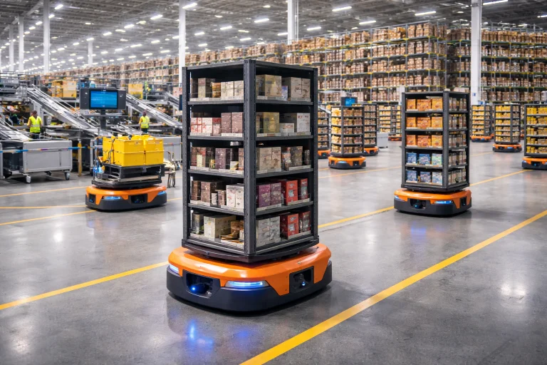
Coordinated multi-agent navigation in a goods-to-person fulfillment environment: differential-drive AMRs transport heavy modular shelving pods through dynamic spatiotemporal reservations managed by real-time fleet software.
Interactive Quick Review: Fleet Coordination & AMRs
Test your understanding of differential-drive kinematics and fleet optimization objectives before exploring motion and scheduling equations:
1. What is the primary engineering focus of warehouse robotics compared to single-robot automation?
2. What mechanism do most warehouse AMRs use to control planar position and orientation?
Kinematic Navigation Model for Differential-Drive AMRs
Most warehouse AMRs utilize differential-drive mechanisms. By actuating the left and right drive wheels with independent linear speeds \(v_L\) and \(v_R\), the vehicle controls its instantaneous forward linear velocity \(v\) and angular turning velocity \(\omega\) in the global warehouse coordinate frame \((X, Y)\).
Let \(L\) denote the wheel track width (distance between wheels) and \(r\) the nominal wheel radius. The planar forward kinematics are governed by the non-holonomic unicycle equations:
$$ \begin{aligned} \dot{x} &= v \cos \theta \\ \dot{y} &= v \sin \theta \\ \dot{\theta} &= \omega \end{aligned} $$where the body velocity vector \([v, \omega]^T\) maps directly from individual wheel angular speeds \([\dot{\phi}_R, \dot{\phi}_L]^T\):
$$ v = \frac{v_R + v_L}{2} = \frac{r(\dot{\phi}_R + \dot{\phi}_L)}{2}, \quad \omega = \frac{v_R - v_L}{L} = \frac{r(\dot{\phi}_R - \dot{\phi}_L)}{L} $$The non-holonomic constraint prevents instantaneous lateral movement along the drive axle:
$$ -\dot{x} \sin \theta + \dot{y} \cos \theta = 0 $$Fleet Coordination, Scheduling, and Makespan Optimization
Rather than optimizing the isolated trajectory of a single vehicle, modern fulfillment fleet management solves multi-agent assignment and routing problems to maximize order handling rates.
Let \(N\) represent the number of operational AMRs, and let \(T_i\) denote the duration required for robot \(i\) to complete its sequence of shelf retrieval, picking station delivery, and pod return operations. The fleet objective seeks to minimize the total completion time (sum of task durations) or the makespan (completion time of the final active task):
$$ \text{Total Flow Time Objective:} \quad \min \sum_{i=1}^N T_i $$ $$ \text{Makespan Objective:} \quad \min \max_{1 \le i \le N} T_i $$Formulations must satisfy dynamic constraints including State-of-Charge (SoC) replenishment cycles, aisle intersection capacities, and time-window delivery deadlines.
Obstacle Avoidance and Spatiotemporal Separation
Warehouse robots share navigation corridors with static structures (racks, sorting tables, pillars) and dynamic agents (peer AMRs, human operators, manual forklifts).
For any two robots \(i\) and \(j\) operating at spatial positions \(\mathbf{p}_i(t) = [x_i(t), y_i(t)]^T\) and \(\mathbf{p}_j(t) = [x_j(t), y_j(t)]^T\), safety requires that their center-to-center Euclidean separation distance remains strictly above the collision safety threshold \(d_{\text{safe}}\):
$$ \|\mathbf{p}_i(t) - \mathbf{p}_j(t)\| = \sqrt{(x_i(t) - x_j(t))^2 + (y_i(t) - y_j(t))^2} \ge d_{\text{safe}} \quad \forall i \ne j, \, \forall t $$where \(d_{\text{safe}} = r_i + r_j + \delta_{\text{margin}}\), incorporating the bounding radii of both vehicles carrying loaded pods plus a dynamic braking margin \(\delta_{\text{margin}}\).
Indoor Industrial Localization Without GPS
Because satellite GNSS signals cannot penetrate steel-reinforced warehouse roofs, AMRs utilize multi-sensor fusion algorithms:
- 2D/3D LiDAR Odometry & SLAM: Continuous laser range measurements match structural corner features against pre-compiled CAD facility floor plans.
- Visual Ground/Ceiling Fiducials: Downward-facing cameras track QR codes or ArUco markers placed at grid intervals on the floor, providing millimeter-accurate global position resets to counteract cumulative wheel drift.
- High-Rate Wheel Odometry & IMU Integration: Optical wheel encoders fused with 6-axis MEMS inertial measurement units via Extended Kalman Filters (EKF) ensure continuous state updates during brief sensor dropouts.
Contemporary 2026 AI-Era Formulations: MAPF and Control Barrier Functions
Modern logistics centers coordinate high-density fleets using scalable multi-agent path finding and real-time safety control algorithms.
1. Multi-Agent Path Finding (MAPF) via Conflict-Based Search (CBS)
When scaling to hundreds of AMRs, decoupled \(A^*\) algorithms fail due to intersection congestion and deadlocks. Conflict-Based Search (CBS) solves two-level hierarchical search problems:
- Low-Level Search: Computes single-agent optimal paths in 3D spacetime \((x, y, t)\) using space-time \(A^*\).
- High-Level Search: Explores a Conflict Tree (CT). When two robots occupy identical spatial grid tiles at time \(t\) (vertex conflict) or cross the same edge simultaneously in opposite directions (edge conflict), the solver introduces temporal constraints that re-route the conflicting robot.
2. Provable Safety with Control Barrier Functions (CBFs)
To safely handle human workers entering AMR transit corridors without conservative emergency stops, robots execute Quadratic Programs (QP) constrained by Control Barrier Functions:
$$ h(\mathbf{p}_i, \mathbf{p}_j) = \|\mathbf{p}_i - \mathbf{p}_j\|^2 - d_{\text{safe}}^2 \ge 0 $$The real-time controller guarantees forward invariance of the safe set \(\mathcal{C}\) by enforcing the derivative condition:
$$ \dot{h}(\mathbf{p}_i, \mathbf{p}_j) + \alpha(h(\mathbf{p}_i, \mathbf{p}_j)) \ge 0 $$where \(\alpha(\cdot)\) is an extended class \(\mathcal{K}_{\infty}\) function, enabling smooth, dynamic deceleration around pedestrians.
Operational Challenges and Failure Modes
Deploying large-scale Autonomous Mobile Robot (AMR) fleets across modern fulfillment centers introduces multifaceted physical, computational, and environmental constraints. Operating hundreds of autonomous units in dense, human-shared industrial corridors exposes several critical failure modes that system architects must mitigate:
-
Rotational Tipping and Dynamic Instability with Elevated Pods:
Goods-to-person AMRs transport payload shelving pods standing up to \(2.5 \text{ m}\) tall and weighing over \(1{,}000 \text{ kg}\). Lifting these structures substantially elevates the combined center of mass (\(h_{\text{com}}\)). During aggressive acceleration, sudden braking, or high-speed in-place pivots, the resultant inertial and centrifugal forces generate severe overturning moments about the outer wheel-ground contact patches. If the lateral acceleration satisfies \(a_{\text{lat}} = v \omega \ge \frac{g L}{2 h_{\text{com}}}\) (where \(L\) is the wheel track width and \(g\) is gravitational acceleration), the pod undergoes rollover instability. Autonomous navigation controllers must enforce dynamic curvature-constrained speed limits and real-time roll-stability bounds. -
Aisle Deadlocks and Spatiotemporal Circular Wait Conditions:
In narrow, single-lane picking corridors, bidirectional travel is structurally impossible. When multiple AMRs arrive simultaneously at perpendicular intersections or attempt to navigate opposing paths through the same aisle, circular dependency graphs emerge. Analogous to Coffman deadlocks in operating systems, each robot reserves a spatial tile while requesting the next tile currently occupied by another waiting agent. Resolving these deadlocks without human intervention requires higher-level Conflict-Based Search (CBS) dispatchers to dynamically assign token priorities, force multi-agent preemption, and designate transient holding spurs. -
Severe Perceptual Occlusion in Dense Storage Racks:
High-density metallic storage racks create continuous physical barriers that block line-of-sight for planar 2D and 3D LiDAR sensors. AMRs turning blindly out of storage rows cannot perceive cross-traffic, manual forklifts, or crossing pedestrians until the front perimeter of the chassis crosses the intersection plane. Furthermore, sensor occlusions degrade scan-matching localization against global facility maps. Mitigating blind-corner hazards requires integrating vehicle-to-infrastructure (V2I) camera networks, corner-mounted millimeter-wave radar, and downward-facing optical fiducial tracking that provides absolute reference positions independently of obstructed horizontal geometry. -
Thermal Degradation and Electrolyte Freezing in Cold-Chain Facilities:
Automated grocery fulfillment often requires robots to operate continuously in deep-freeze environments maintained at \(-20^\circ\text{C}\) to \(-25^\circ\text{C}\). At these sub-zero temperatures, internal lithium-ion battery impedance escalates dramatically, cutting effective operational capacity and discharge runtime by \(40\%\) to \(50\%\) while drastically extending recharge durations. Furthermore, standard industrial drive gear lubricants freeze or thicken, causing excessive motor current draws, wheel-torque imbalances, and premature gearbox failure. Cold-chain AMRs require specialized closed-loop internal resistance heating blankets, winterized synthetic fluorinated greases, and hermetically sealed IP65/IP67 enclosures to prevent internal condensation and electronic short circuits during transition cycles between ambient dock areas and frozen picking vaults.
Interactive Quick Review: Kinematics, Scheduling & Safety
Reinforce key concepts regarding differential-drive kinematics, task scheduling objectives, and safe separation constraints before reviewing the FAQ:
1. What is the primary optimization objective in warehouse fleet task scheduling?
2. What mathematical condition defines safe inter-robot obstacle avoidance?
External References and Further Reading
Consult the following industry white papers and peer-reviewed journals for advanced study in automated material handling:
- MHI (Material Handling Industry) – Solutions Community – Industry standards, automated material handling whitepapers, and AMR logistics metrics.
- IEEE Transactions on Automation Science and Engineering – Foundational research covering Multi-Agent Path Finding (MAPF), Automated Guided Vehicle routing, and warehouse dispatch algorithms.
- Amazon Science – Robotics & Fulfillment Research – Academic publications detailing goods-to-person fulfillment, robotic manipulation, and large-scale fleet orchestration.
Frequently Asked Questions about Warehouse Robotics and AMRs
What differentiates an AGV from an AMR in warehouse environments?
Automated Guided Vehicles (AGVs) follow rigid physical paths (magnetic tape, embedded wires, optical floor markers) and stop when an obstacle blocks their path. Autonomous Mobile Robots (AMRs) build onboard environmental maps using LiDAR and SLAM, allowing them to dynamically replan paths around unexpected obstacles.
How do fleet managers solve Multi-Agent Path Finding (MAPF) in real time?
Fleet systems use algorithms such as Conflict-Based Search (CBS) or windowed hierarchical planners. By reserving space-time nodes \((x, y, t)\), the software detects trajectory intersections and assigns priority rules or temporal holding patterns to maintain collision-free travel.
Why is zero-radius turning crucial for logistics mobile bases?
Fulfillment centers maximize storage capacity by using narrow aisles. Differential-drive AMRs can rotate 360 degrees about their central axle, allowing them to reverse direction or enter cross-aisles without requiring wide turning envelopes.
How do AMRs maintain millimeter precision under accumulated odometry drift?
While high-speed wheel encoders accumulate position error from wheel slip, downward-facing optical sensors continuously read ground fiducial markers (QR/DataMatrix codes). Each marker provides an absolute coordinate fix that resets cumulative odometry error.
How are autonomous charging schedules optimized across large fleets?
Predictive battery fleet management systems monitor real-time State-of-Charge (SoC). Robots are routed to charging pads or automated battery-swap stations during operational lulls, ensuring enough active robots remain deployed to meet fulfillment quotas.
How do AMRs ensure human worker safety during shared-aisle picking?
Robots carry certified safety LiDAR scanners configured with dual safety zones. Penetration of an outer detection field triggers gradual deceleration, while violation of an inner zone activates a fail-safe emergency stop.
What are the main economic drivers for adopting goods-to-person AMRs?
Goods-to-person automation eliminates manual walking time in warehouses, which can account for up to 60–70% of a picker's shift. Transporting inventory pods directly to workstations can increase order picking rates by 300% to 500%.
What technical specializations prepare engineers for warehouse robotics?
Core foundational skills include non-holonomic mobile robotics kinematics, operations research, spatial graph search algorithms (MAPF / \(A^*\)), ROS 2 navigation stacks (Nav2), and distributed system architectures.
End-of-Page Exercises: Review, Conceptual Analysis & Derivations
Part I: Review Questions
1. What kinematic differential equations model planar motion for a differential-drive AMR?
2. What objective function models fleet scheduling optimization in fulfillment centers?
3. What inequality enforces safe Euclidean distance separation between two warehouse robots?
4. Why is satellite GPS unusable for indoor warehouse localization?
5. How is global fleet state \(S(t)\) updated in centralized management software?
6. Name four primary logistics application sectors for mobile robots.
7. What navigation capability distinguishes an AMR from an AGV?
8. What defines the "goods-to-person" paradigm in automated fulfillment?
9. List three major operational bottlenecks in high-density AMR fleets.
10. Name five foundational university disciplines essential for warehouse robotics engineering.
Part II: Thought-Provoking Conceptual Questions
1. Why do Multi-Agent Path Finding (MAPF) algorithms face exponential computational complexity as fleet size \(N\) scales?
2. How does transitioning from magnetic-tape AGVs to flexible AMRs alter warehouse architectural planning?
3. What safety trade-offs emerge when increasing AMR operational speeds from \(1.0 \text{ m}\cdot\text{s}^{-1}\) to \(2.5 \text{ m}\cdot\text{s}^{-1}\)?
4. Why can centralized cloud fleet control trigger widespread operational failure during Wi-Fi network partitions?
5. How do center-of-mass shifts affect the cornering stability of differential-drive AMRs carrying heavy pods?
6. In what ways does cold-storage logistics (-20°C) constrain mobile robot hardware design?
7. Why are intersection deadlocks in warehouse aisles analogous to operating system resource deadlocks?
8. How do predictive maintenance telemetry streams reduce unplanned downtime across large fleets?
9. What operational trade-offs balance human picker privacy against fleet throughput optimization?
10. Why do urban micro-fulfillment centers require higher AMR operating densities than regional distribution hubs?
11. How does extrinsic sensor calibration drift affect long-term SLAM map consistency?
12. What capital investment metrics determine the financial breakeven of AMR automation?
Part III: Step-by-Step Numerical Engineering Derivations
Problem 1: Differential-Drive Kinematic Forward Trajectory
Scenario: A warehouse AMR starts at origin \([x_0, y_0]^T = [0.0, 0.0]^T \text{ m}\) with heading angle \(\theta_0 = 0.0 \text{ rad}\). The vehicle travels with constant linear forward velocity \(v = 1.50 \text{ m}\cdot\text{s}^{-1}\) and zero angular velocity (\(\omega = 0\)) for duration \(t = 10.0 \text{ s}\). Derive the final Cartesian coordinates \(x(t)\) and \(y(t)\).
Step-by-Step Derivation:
$$ \begin{aligned} x(t) &= x_0 + \int_0^t v \cos\theta(\tau) \, d\tau = 0.0 + \int_0^{10.0} 1.50 \cos(0) \, d\tau \\ &= 1.50 \times 10.0 = 15.0 \text{ m} \\ y(t) &= y_0 + \int_0^t v \sin\theta(\tau) \, d\tau = 0.0 + \int_0^{10.0} 1.50 \sin(0) \, d\tau \\ &= 0.0 \text{ m} \end{aligned} $$Answer & Conclusion: The final coordinates are \(x_{\text{final}} = 15.0 \text{ m}\) and \(y_{\text{final}} = 0.0 \text{ m}\).
Problem 2: Fleet Scheduling Makespan and Flow-Time Redistribution
Scenario: A dispatcher schedules tasks across \(N = 3\) AMRs. Baseline completion times are \(T_1 = 25.0 \text{ s}\), \(T_2 = 45.0 \text{ s}\), and \(T_3 = 80.0 \text{ s}\). A heuristic reassignment redistributes tasks such that \(T_1' = 35.0 \text{ s}\), \(T_2' = 40.0 \text{ s}\), and \(T_3' = 55.0 \text{ s}\). Calculate total flow time reduction and makespan reduction.
Step-by-Step Derivation:
$$ \begin{aligned} \text{Baseline Total Flow Time} &= 25.0 + 45.0 + 80.0 = 150.0 \text{ s} \\ \text{Optimized Total Flow Time} &= 35.0 + 40.0 + 55.0 = 130.0 \text{ s} \\ \Delta T_{\text{flow}} &= 150.0 - 130.0 = 20.0 \text{ s saved} \quad \left(\frac{20.0}{150.0} \times 100\% \approx 13.33\%\right) \\ \text{Baseline Makespan } M_{\text{base}} &= \max(25, 45, 80) = 80.0 \text{ s} \\ \text{Optimized Makespan } M_{\text{opt}} &= \max(35, 40, 55) = 55.0 \text{ s} \\ \Delta M &= 80.0 - 55.0 = 25.0 \text{ s reduction} \quad \left(\frac{25.0}{80.0} \times 100\% = 31.25\%\right) \end{aligned} $$Answer & Conclusion: Total flow time improves by \(13.33\%\) and fleet makespan drops from \(80.0 \text{ s}\) to \(55.0 \text{ s}\) (a \(31.25\%\) acceleration).
Problem 3: Inter-Robot Euclidean Safety Separation Verification
Scenario: In an intersection corridor, AMR 1 is at \(\mathbf{p}_1 = [4.20, 8.50]^T \text{ m}\) and AMR 2 is at \(\mathbf{p}_2 = [5.80, 7.30]^T \text{ m}\). Safe separation policy requires \(d_{\text{safe}} = 2.00 \text{ m}\). Calculate the Euclidean distance \(\|\mathbf{p}_1 - \mathbf{p}_2\|\) and verify the safety constraint.
Step-by-Step Derivation:
$$ \begin{aligned} \Delta x &= 4.20 - 5.80 = -1.60 \text{ m} \\ \Delta y &= 8.50 - 7.30 = +1.20 \text{ m} \\ \|\mathbf{p}_1 - \mathbf{p}_2\| &= \sqrt{(-1.60)^2 + (1.20)^2} = \sqrt{2.56 + 1.44} = \sqrt{4.00} = 2.00 \text{ m} \\ \|\mathbf{p}_1 - \mathbf{p}_2\| &\ge d_{\text{safe}} \quad \Rightarrow \quad 2.00 \text{ m} \ge 2.00 \text{ m} \quad (\text{Constraint Satisfied Exactly}) \end{aligned} $$Answer & Conclusion: The distance is exactly \(2.00 \text{ m}\), meeting the boundary condition of the safety threshold.
Problem 4: Daily Fleet Energy Consumption and Duty Cycle Sizing
Scenario: An AMR operates across a \(16.0\text{-hour}\) shift, drawing average electrical power \(P_{\text{avg}} = 350.0 \text{ W}\). Battery packs have usable capacity \(E_{\text{cap}} = 1{,}400.0 \text{ Wh}\) (\(1.40 \text{ kWh}\)). Calculate total consumed energy and determine the required full charge-discharge cycles per shift.
Step-by-Step Derivation:
$$ \begin{aligned} E_{\text{total}} &= P_{\text{avg}} \times t_{\text{shift}} = 350.0 \text{ W} \times 16.0 \text{ h} = 5{,}600.0 \text{ Wh} = 5.60 \text{ kWh} \\ N_{\text{cycles}} &= \frac{E_{\text{total}}}{E_{\text{cap}}} = \frac{5{,}600.0 \text{ Wh}}{1{,}400.0 \text{ Wh/cycle}} = 4.00 \text{ cycles} \end{aligned} $$Answer & Conclusion: Total consumed energy is \(5.60 \text{ kWh}\), requiring \(4.0\) equivalent full battery charging cycles per shift.
Problem 5: Aisle Traversal Transit Time and Shift Throughput
Scenario: An AMR navigates a straight picking aisle of length \(D = 50.0 \text{ m}\) at constant cruise velocity \(v = 1.25 \text{ m}\cdot\text{s}^{-1}\). Calculate single trip transit time \(t_{\text{trip}}\). If the robot completes \(N_{\text{trips}} = 120\) picking runs during a shift, find total active transit time in minutes.
Step-by-Step Derivation:
$$ \begin{aligned} t_{\text{trip}} &= \frac{D}{v} = \frac{50.0 \text{ m}}{1.25 \text{ m}\cdot\text{s}^{-1}} = 40.0 \text{ s} \\ t_{\text{shift, sec}} &= N_{\text{trips}} \times t_{\text{trip}} = 120 \times 40.0 \text{ s} = 4{,}800.0 \text{ s} \\ t_{\text{shift, min}} &= \frac{4{,}800.0}{60.0} = 80.0 \text{ min} \quad (1.33 \text{ h}) \end{aligned} $$Answer & Conclusion: A single run requires \(40.0 \text{ s}\), accumulating \(80.0 \text{ minutes}\) of travel across \(120\) trips.
Problem 6: Centralized Fleet Telemetry Bandwidth Sizing
Scenario: A centralized fleet server monitors \(N = 250\) active AMRs. Each vehicle sends state packets of size \(S = 256 \text{ bytes}\) at an update frequency \(f = 2.0 \text{ Hz}\). Determine total incoming network throughput in Kilobytes per second (KB/s) and Megabits per second (Mbps).
Step-by-Step Derivation:
$$ \begin{aligned} R_{\text{single}} &= 256 \text{ bytes} \times 2.0 \text{ s}^{-1} = 512.0 \text{ bytes/s} \\ B_{\text{fleet, bytes}} &= 250 \times 512.0 \text{ bytes/s} = 128{,}000.0 \text{ bytes/s} \\ B_{\text{fleet, KB/s}} &= \frac{128{,}000.0}{1{,}000} = 128.0 \text{ KB/s} \\ B_{\text{fleet, Mbps}} &= \frac{128{,}000.0 \times 8 \text{ bits/byte}}{10^6} = 1.024 \text{ Mbps} \end{aligned} $$Answer & Conclusion: Fleet state telemetry requires \(128.0 \text{ KB/s}\) (\(1.024 \text{ Mbps}\)) of continuous network bandwidth.
Problem 7: Storage Density Increase via Aisle Width Reduction
Scenario: Manual forklift facilities require aisle widths \(W_{\text{manual}} = 3.50 \text{ m}\). Transitioning to compact-footprint AMRs allows aisle width reduction to \(W_{\text{amr}} = 1.50 \text{ m}\). Calculate aisle footprint percentage savings and the floor space efficiency multiplier.
Step-by-Step Derivation:
$$ \begin{aligned} \Delta W &= W_{\text{manual}} - W_{\text{amr}} = 3.50 \text{ m} - 1.50 \text{ m} = 2.00 \text{ m} \\ \text{Percentage Reduction} &= \frac{2.00}{3.50} \times 100\% \approx 57.14\% \\ \text{Efficiency Multiplier} &= \frac{W_{\text{manual}}}{W_{\text{amr}}} = \frac{3.50}{1.50} \approx 2.33\times \end{aligned} $$Answer & Conclusion: Aisle space is reduced by \(57.14\%\), delivering a \(2.33\times\) improvement in footprint utilization.
Problem 8: Differential-Drive Inverse Kinematics for In-Place Rotation
Scenario: A differential AMR has track width \(L = 0.50 \text{ m}\). The vehicle executes a pure in-place rotation with angular velocity \(\omega = 1.00 \text{ rad}\cdot\text{s}^{-1}\) and zero linear forward velocity (\(v = 0\)). Calculate required tangential wheel velocities \(v_R\) and \(v_L\).
Step-by-Step Derivation:
$$ \begin{aligned} v_R &= v + \frac{\omega L}{2} = 0.0 + \frac{1.00 \times 0.50}{2} = +0.25 \text{ m}\cdot\text{s}^{-1} \\ v_L &= v - \frac{\omega L}{2} = 0.0 - \frac{1.00 \times 0.50}{2} = -0.25 \text{ m}\cdot\text{s}^{-1} \end{aligned} $$Answer & Conclusion: In-place rotation requires the right wheel to drive forward at \(+0.25 \text{ m}\cdot\text{s}^{-1}\) and the left wheel to reverse at \(-0.25 \text{ m}\cdot\text{s}^{-1}\).
Problem 9: Fulfillment Picking Throughput Acceleration Factor
Scenario: A manual picking zone fulfills \(Q_{\text{manual}} = 400\) order lines per shift. Deploying an automated goods-to-person AMR system increases output to \(Q_{\text{amr}} = 1{,}800\) lines per shift. Determine the net throughput increase \(\Delta Q\) and the throughput multiplier.
Step-by-Step Derivation:
$$ \begin{aligned} \Delta Q &= Q_{\text{amr}} - Q_{\text{manual}} = 1{,}800 - 400 = 1{,}400 \text{ lines/shift} \\ \text{Throughput Multiplier} &= \frac{Q_{\text{amr}}}{Q_{\text{manual}}} = \frac{1{,}800}{400} = 4.50\times \end{aligned} $$Answer & Conclusion: Output increases by \(1{,}400\) orders per shift, representing a \(4.50\times\) throughput gain.
Problem 10: Spatiotemporal Intersection Clearance and Queue Distance
Scenario: Two AMRs approach a 4-way aisle intersection at speed \(v = 1.00 \text{ m}\cdot\text{s}^{-1}\). Robot 1 traverses the intersection zone, blocking cross-traffic for duration \(\tau_{\text{block}} = 3.50 \text{ s}\). Calculate the minimum spatial queueing distance \(d_{\text{queue}}\) Robot 2 must reserve before the intersection to come to a stop without entering the conflict zone.
Step-by-Step Derivation:
$$ \begin{aligned} d_{\text{queue}} &= v \times \tau_{\text{block}} = 1.00 \text{ m}\cdot\text{s}^{-1} \times 3.50 \text{ s} = 3.50 \text{ m} \end{aligned} $$Answer & Conclusion: Robot 2 requires a \(3.50 \text{ m}\) queueing buffer to safely wait out the intersection occupancy.
Problem 11: 2D Safety LiDAR Point-Cloud Stream Bandwidth
Scenario: An AMR navigation LiDAR spins at scan frequency \(f_{\text{scan}} = 10.0 \text{ Hz}\). Each revolution captures \(N_p = 32{,}000\) measurement points. Each point encodes 3D Cartesian coordinates using three 32-bit floating-point numbers (\(3 \times 4 \text{ bytes} = 12 \text{ bytes}\)). Calculate generated scan packet size and data stream bandwidth in Megabytes per second (MB/s).
Step-by-Step Derivation:
$$ \begin{aligned} S_{\text{rev}} &= 32{,}000 \text{ points} \times 12 \text{ bytes/point} = 384{,}000 \text{ bytes} = 384.0 \text{ KB} \\ B_{\text{stream}} &= 384{,}000 \text{ bytes/rev} \times 10.0 \text{ rev/s} = 3{,}840{,}000 \text{ bytes/s} \\ B_{\text{stream, MB/s}} &= \frac{3{,}840{,}000}{10^6} = 3.84 \text{ MB/s} \end{aligned} $$Answer & Conclusion: The sensor produces \(384.0 \text{ KB}\) per revolution, yielding a streaming throughput of \(3.84 \text{ MB/s}\).
Problem 12: Automated Charging Station Contention Factor
Scenario: A logistics zone contains \(N_{\text{fleet}} = 40\) AMRs served by \(N_{\text{docks}} = 5\) automated charging stations. Each robot requires one \(30.0\text{-minute}\) recharge during an \(8.0\text{-hour}\) operating block. Calculate the dock contention factor and the required charging dock utilization ratio.
Step-by-Step Derivation:
$$ \begin{aligned} \text{Dock Contention Ratio} &= \frac{N_{\text{fleet}}}{N_{\text{docks}}} = \frac{40}{5} = 8.0\times \\ T_{\text{charge, total}} &= 40 \times 0.50 \text{ h} = 20.0 \text{ dock-hours required} \\ T_{\text{dock, available}} &= 5 \text{ docks} \times 8.0 \text{ h} = 40.0 \text{ dock-hours available} \\ \text{Utilization Factor } U &= \frac{T_{\text{charge, total}}}{T_{\text{dock, available}}} = \frac{20.0}{40.0} = 0.50 \quad (50.0\%) \end{aligned} $$Answer & Conclusion: The fleet maintains an \(8.0\times\) robot-to-dock ratio with a \(50.0\%\) charging dock utilization factor, confirming that staggered scheduling will avoid charging queues.
Warehouse Robotics and Autonomous Mobile Robots (AMRs) — Summary & Wrap-Up
Warehouse logistics robotics demonstrates how non-holonomic mobile kinematics, multi-agent path finding (MAPF), and cloud fleet orchestration work together to automate large-scale material handling. Differential-drive kinematic models (\(\dot{x} = v \cos \theta, \dot{y} = v \sin \theta\)), fleet makespan optimization, and Euclidean separation constraints ensure collision-free movement in high-density facilities. Fusing LiDAR SLAM with floor fiducial markers eliminates accumulated odometry drift without satellite GPS.
As logistics centers expand, modern methods—such as Conflict-Based Search (CBS) in 3D spacetime and Control Barrier Functions (CBFs)—provide scalable traffic routing and human-robot safety, delivering high reliability across modern automated fulfillment operations.