
Modern robots are rarely controlled by a single monolithic computer. Instead, perception pipelines, real-time control processors, sensor aggregation hubs, low-level motor drivers, and offboard cloud clusters operate across physically separated hardware targets that exchange telemetry and control streams across heterogeneous networks. Robotics middleware provides the structured, abstracted communication backbone that enables these distributed computational nodes to function as a unified physical system.
Without standardized middleware, every software module would need to implement bespoke socket handling, serialization logic, byte alignment protocols, and thread synchronization barriers. Such tightly coupled systems become fragile, difficult to debug, and mathematically intractable to scale. Middleware solves this architectural bottleneck by decoupling producers and consumers of information, allowing robotics engineers to focus on state estimation, path planning, and non-linear control rather than low-level socket programming.
Within the robotics software stack, middleware forms the core transport fabric connecting high-fidelity simulation engines, real-time embedded motor controllers, distributed edge nodes, and centralized fleet intelligence. It converts isolated robotic algorithms into scalable, fault-tolerant distributed intelligence.
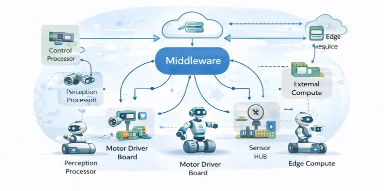
This architecture illustrates how modern robotics distributes computation across specialized physical domains. High-bandwidth perception nodes process camera streams and LiDAR clouds on dedicated edge GPUs, low-latency microcontrollers execute deterministic 1 kHz joint feedback loops, and remote cloud infrastructure evaluates fleet logistics and predictive digital twins. The middleware layer coordinates message serialization, bus routing, and quality-of-service enforcement, ensuring modularity without compromising control loop determinism.
Interactive Quick Review: Distributed Architecture & Middleware
Test your understanding of distributed robotic nodes and network abstraction before exploring communication graph mathematics:
1. What is the primary role of robotics middleware in distributed multi-processor systems?
Answer: Middleware provides a standardized, decoupled communication abstraction layer that manages network protocols, message serialization, and timing synchronization, enabling specialized processors (perception, planning, motor actuation) to coordinate as an integrated system without point-to-point socket coupling.
2. How does loose coupling improve overall system reliability in a distributed robot?
Answer: Loose coupling enforces process memory isolation. A software crash, memory leak, or driver stall in a high-level non-critical module (such as a 3D vision object detector) cannot corrupt the memory space or halt the execution of safety-critical embedded motor control loops.
Glossary of Key Terminology
Essential definitions governing distributed computing graphs, network transport protocols, and real-time middleware coordination:
Distributed Network Architecture & Graph Modeling
Modern robotics organizes compute into distributed networks modeled rigorously via algebraic graph theory. Let the robotic network be represented as a directed or undirected graph:
$$\mathcal{G} = (\mathcal{V}, \mathcal{E})$$where \(\mathcal{V} = \{v_1, v_2, \dots, v_n\}\) denotes the set of \(n\) computational vertices (embedded microcontrollers, GPU perception accelerators, edge nodes, and cloud dispatchers), and \(\mathcal{E} \subseteq \mathcal{V} \times \mathcal{V}\) represents active communication channels. An edge \((v_i, v_j) \in \mathcal{E}\) indicates that node \(j\) can receive information directly from node \(i\).
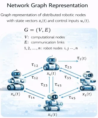
The network connectivity is algebraically encoded by the Adjacency Matrix \(\mathbf{A} = [a_{ij}] \in \mathbb{R}^{n \times n}\), where \(a_{ij} > 0\) if \((v_j, v_i) \in \mathcal{E}\), and \(a_{ij} = 0\) otherwise. The Degree Matrix \(\mathbf{D} = \text{diag}(d_1, d_2, \dots, d_n)\) contains the in-degrees \(d_i = \sum_{j=1}^n a_{ij}\). The Graph Laplacian Matrix \(\mathbf{L}\) is defined as:
$$\mathbf{L} = \mathbf{D} - \mathbf{A}$$The spectral properties of \(\mathbf{L}\) govern information propagation across the robotic network. Specifically, the second smallest eigenvalue of \(\mathbf{L}\), known as the algebraic connectivity or Fiedler eigenvalue \(\lambda_2(\mathbf{L})\), dictates the convergence rate of consensus algorithms, multi-agent synchronization, and distributed state estimation across the robot.
Message Passing Dynamics, Latency & Transport Delays
When physical states or actuation commands traverse network channels, message transmission is subject to communication delays composed of packet serialization, transport propagation, routing switches, and receiver queue buffering. When node \(i\) transmits state \(\mathbf{x}_i(t)\) to node \(j\), the state available to node \(j\) incorporates transport delay \(\tau_{ij}\):
$$\mathbf{x}_j(t) = \mathbf{x}_i(t - \tau_{ij})$$In closed-loop feedback systems, transport delay introduces an uncompensated phase lag \(\phi_{\text{lag}} = \omega \tau_{ij}\) into the open-loop transfer function. For continuous motion control, this degrades the phase margin \(\Phi_m\). If transmission latency exceeds the controller sampling period \(T_s\):
$$\tau_{ij} \ge T_s$$the controller operates on stale feedback telemetry. In high-bandwidth dynamic robots (e.g., quadruped balancing or aerial manipulation), uncompensated message delays lead to overshoot, command oscillations, and closed-loop instability.
Distributed Consensus & State Synchronization
When multiple processors or autonomous fleet agents must agree on a shared coordinate frame, heading angle, or environmental map without relying on a centralized server, they execute distributed consensus algorithms. The continuous-time consensus protocol across graph \(\mathcal{G}\) follows the dynamic differential equation:
$$\dot{\mathbf{x}}_i(t) = \sum_{j \in \mathcal{N}_i} a_{ij} \left( \mathbf{x}_j(t) - \mathbf{x}_i(t) \right)$$where \(\mathcal{N}_i = \{v_j \in \mathcal{V} : (v_j, v_i) \in \mathcal{E}\}\) is the set of active neighbors communicating with node \(i\). Stacking states across all \(n\) nodes yields the compact vector dynamic equation:
$$\dot{\mathbf{x}}(t) = -\mathbf{L} \mathbf{x}(t)$$For discrete-time embedded implementation with step size \(\epsilon > 0\), nodes execute the iterative update rule:
$$\mathbf{x}_i^{k+1} = \mathbf{x}_i^k + \epsilon \sum_{j \in \mathcal{N}_i} a_{ij} \left( \mathbf{x}_j^k - \mathbf{x}_i^k \right)$$If the communication graph \(\mathcal{G}\) is undirected and connected, and step size satisfies \(0 < \epsilon < 1/\max_i(d_i)\), all nodes asymptotically converge to the exact
$$\lim_{k \to \infty} \mathbf{x}_i^k = \frac{1}{n} \sum_{j=1}^n \mathbf{x}_j^0$$Engineering Challenges & Technical Solutions
Deploying distributed robotics middleware across physical machines, wireless industrial environments, and embedded processors introduces several structural and operational challenges:
The Challenge: High-bandwidth sensors (4K visual cameras, 128-beam 3D LiDAR point clouds) produce tens of megabytes per message. Serializing C++ object trees into Common Data Representation (CDR) byte streams and copying buffers between kernel and user memory consumes massive CPU overhead and adds multi-millisecond latency.
- Zero-Copy Shared Memory IPC: Implementing shared-memory mechanisms (such as Eclipse iceoryx or POSIX shared memory) that transfer raw memory pointers between processes on the same host, dropping IPC latency to sub-microsecond levels.
- FlatBuffers and Zero-Serialization Schemas: Utilizing binary data formats where data can be accessed directly in its serialized buffer without unpacking, eliminating decoding overhead.
The Challenge: Industrial Wi-Fi and 5G connections experience multipath interference, transmission retries, and network congestion. Unpredictable timing jitter causes state packets to arrive out of order or clump together, breaking timing assumptions in discrete controllers.
- Time-Triggered Transport & TSN: Deploying Time-Sensitive Networking over industrial Ethernet switches to enforce bounded worst-case latency via scheduled time slots.
- Predictor-Observer State Estimators: Using model-based Kalman filters or Smith Predictors inside the receiving node to forward-propagate system states during packet bursts, as covered in Real-Time Embedded Systems in Robotics.
The Challenge: Plaintext multicast discovery and unencrypted communication allow unauthorized devices on the local network to intercept proprietary sensor topics, eavesdrop on camera feeds, or inject malicious velocity setpoints directly to actuators.
- SROS 2 & DDS-Security Extensions: Enforcing mutual X.509 PKI certificate authentication, encrypting packet payloads via AES-GCM (128/256-bit), and signing topic permissions via governance XML files, detailed in Robot Operating System (ROS and ROS 2).
- VLAN Hardware Segmentation: Electrically isolating safety-critical fieldbuses (CANopen, EtherCAT) from general-purpose wireless teleoperation networks using managed industrial network switches.
The Challenge: Separate hardware clocks on embedded cameras, LiDAR units, and IMUs drift by milliseconds over time due to temperature changes and oscillator tolerances. Fusing misaligned sensor data introduces spatial registration errors in SLAM and state estimation.
- Precision Time Protocol (IEEE 1588 PTP): Synchronizing internal hardware timers across network interfaces to sub-microsecond precision via hardware-level packet timestamping.
- Hardware Trigger Synchronization: Driving camera exposure strobes and LiDAR firing pulses via a shared physical PWM trigger line sourced from a central master clock.
Fault Tolerance & Triple Modular Redundancy (TMR)
Safety-critical autonomous systems (e.g., autonomous vehicles, surgical manipulators, space robotics) must continue operating safely despite hardware faults, power interruptions, or memory corruption. Fault tolerance is established through physical hardware redundancy and voting algorithms.
Consider a system incorporating \(R\) identical redundant backup compute nodes operating in parallel with an active primary node (total \(R+1\) nodes). Assuming each node fails independently with probability \(p \in (0, 1)\), the overall system failure probability \(P_{\text{fail}}\) requires all \(R+1\) nodes to fail simultaneously:
$$P_{\text{fail}} = p^{R+1}$$The resulting system reliability \(P_{\text{system}}\) is formulated as:
$$P_{\text{system}} = 1 - P_{\text{fail}} = 1 - p^{R+1}$$Triple Modular Redundancy (TMR) Voting Dynamics
In a Triple Modular Redundancy (TMR) configuration (\(N = 3\) nodes), all three processors execute the identical control algorithm concurrently. A majority voter circuit or software consensus arbiter evaluates outputs using a 2-out-of-3 majority rule. The system functions correctly if at least two processors agree. The overall failure probability occurs if two or three nodes fail simultaneously:
$$P_{\text{fail, TMR}} = {3 \choose 2} p^2 (1 - p) + {3 \choose 3} p^3 = 3p^2(1 - p) + p^3 = 3p^2 - 2p^3$$The resulting TMR reliability becomes:
$$P_{\text{TMR}} = 1 - P_{\text{fail, TMR}} = 1 - 3p^2 + 2p^3$$For independent failure rates \(p < 0.5\), TMR substantially reduces system failure risk relative to a single processor architecture.
Interactive Quick Review: Consensus, QoS & Real-Time Constraints
Reinforce key concepts regarding average consensus, real-time latency bounds, and fault-tolerant redundancy before reviewing the FAQ:
1. How does the average consensus update rule \(\mathbf{x}_i^{k+1} = \mathbf{x}_i^k + \epsilon \sum a_{ij}(\mathbf{x}_j^k - \mathbf{x}_i^k)\) achieve distributed agreement?
Answer: Each node iteratively adjusts its state by adding a weighted sum of the differences between its own state and its neighbors' states. Driven by the spectral properties of the Graph Laplacian (\(\mathbf{L} = \mathbf{D} - \mathbf{A}\)), this drives all connected nodes toward the global mean without central arbitration.
2. What condition must be satisfied by total latency (\(T_c + T_n\)) to ensure real-time closed-loop control stability?
Answer: Total worst-case execution time (node computation \(T_c\) plus network transport delay \(T_n\)) must remain strictly less than or equal to the control sampling period: \(T_c + T_n \le T_s\).
External References and Further Reading
To explore middleware standards, distributed network theory, and industrial communication protocols, consult the following authoritative sources:
- Object Management Group (OMG) DDS Specification – Official international standard for the Data Distribution Service publish-subscribe protocol used in real-time distributed control systems.
- ROS 2 Documentation & Design Architecture – Developer guides covering distributed computation graphs, inter-process communication, zero-copy shared memory, and Quality of Service (QoS) parameters.
- IEEE Transactions on Control of Network Systems – Academic research on multi-agent consensus protocols, graph-theoretic control, and distributed stabilization over delayed communication networks.
Frequently Asked Questions about Robotics Middleware and Distributed Systems
What is the difference between ROS 1 and ROS 2 middleware architectures?
ROS 1 relies on a centralized Master node (roscore) for registration and uses custom socket protocols (TCPROS/UDPROS). ROS 2 replaces this master with the decentralized, industry-standard Data Distribution Service (DDS), enabling peer-to-peer discovery, configurable QoS policies, real-time determinism, and built-in TLS/DTLS encryption.
Why is the publish–subscribe model preferred over client–server for sensor data streaming?
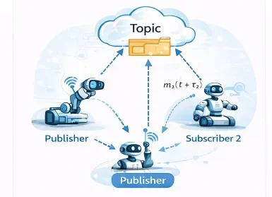
Publish-subscribe provides asynchronous, many-to-many communication that completely decouples message producers from consumers. A sensor node publishes readings at a fixed rate without waiting for requests, allowing perception, logging, and safety modules to process data concurrently without blocking the sensor pipeline.
How do network communication delays (\(\tau_{ij}\)) cause feedback control instability?
Communication latency introduces transport phase lag into the feedback path (\(\phi_{\text{lag}} = \omega \tau_{ij}\)). Late telemetry forces controllers to apply forces based on outdated system states, leading to over-correction, high-frequency limit-cycle oscillations, and loss of phase margin.
What is the difference between Strong Consistency and Eventual Consistency in distributed robots?
Strong consistency guarantees that all nodes observe an identical state simultaneously, requiring distributed blocking locks that increase communication latency. Eventual consistency allows temporary state differences between nodes, guaranteeing they converge to identical values over time while allowing local nodes to proceed without blocking.
What is zero-copy message passing in modern robotics middleware?
Zero-copy messaging allows nodes executing within the same physical memory space to exchange data by passing pointer references to shared memory blocks rather than serializing and copying bytes across process boundaries, lowering transport latency to sub-microsecond levels.
How do distributed consensus algorithms manage swarm robotics coordination?
Consensus algorithms allow independent robots in a swarm to converge on shared target headings, formations, or task allocations via local neighbor-to-neighbor communication updates (\(\mathbf{x}_i^{k+1} = \mathbf{x}_i^k + \epsilon \sum a_{ij}(\mathbf{x}_j^k - \mathbf{x}_i^k)\)), eliminating the need for a central coordinator.
End-of-Page Exercises: Review, Thought-Provoking & Engineering Problems
Section 1: Foundational Review Questions & Answers
1. How is a distributed robotic network represented mathematically in graph theory?
Answer: As a graph \(\mathcal{G} = (\mathcal{V}, \mathcal{E})\), where \(\mathcal{V}\) represents the set of computational nodes and \(\mathcal{E}\) represents the set of directional or bidirectional communication channels.
2. What mathematical expression models the state received at node j from node i under communication delay \(\tau_{ij}\)?
Answer: \(\mathbf{x}_j(t) = \mathbf{x}_i(t - \tau_{ij})\).
3. What formula determines required network bandwidth \(B_{\text{required}}\) for a streaming sensor topic?
Answer: \(B_{\text{required}} = S \times f\), multiplying message payload size in bits by transmission frequency in Hz.
4. How does the publish–subscribe communication pattern decouple system components?
Answer: Publishers send messages to named topics without target address awareness, allowing subscribers to receive data independently without modifying the publisher node.
5. What is the fundamental discrete update equation for an average consensus algorithm on node i?
Answer: \(\mathbf{x}_i^{k+1} = \mathbf{x}_i^k + \epsilon \sum_{j \in \mathcal{N}_i} a_{ij}(\mathbf{x}_j^k - \mathbf{x}_i^k)\).
6. How is overall system reliability \(P_{\text{system}}\) modeled when deploying R redundant backup nodes with node failure probability p?
Answer: \(P_{\text{system}} = 1 - p^{R+1}\).
7. What inequality enforces the real-time execution constraint across a distributed network link?
Answer: \(T_c + T_n \le T_s\), ensuring computation time plus network transport delay does not exceed the control sampling period.
8. What trade-offs differentiate cloud computing from edge computing in robotic architectures?
Answer: Cloud computing offers vast computational capacity for global fleet optimization at the cost of higher network latency; edge computing delivers low-latency processing close to hardware with constrained local compute resources.
9. What middleware technology underpinning ROS 2 provides peer-to-peer node discovery?
Answer: Data Distribution Service (DDS).
10. Name four fundamental engineering trade-offs faced when designing robotics middleware.
Answer: Throughput vs. latency, strong consistency vs. scalability, hardware redundancy vs. cost/weight, and cryptographic security vs. real-time execution overhead.
Section 2: Analytical & Thought-Provoking Questions
1. How does message serialization introduce computational latency during high-frequency data transmission?
Answer: Serialization traverses memory structures to encode variables into architecture-agnostic binary streams (such as CDR or Protocol Buffers). For complex multi-field messages or large arrays (such as 3D point clouds), CPU cycles spent performing memory traversal and endian conversions add multi-millisecond latency to the processing pipeline.
2. Why can network packet drops in wireless multi-robot swarms break mathematical convergence in consensus algorithms?
Answer: Consensus convergence requires a connected communication graph \(\mathcal{G}\). Packet loss dynamically severs communication edges \(\mathcal{E}\). If loss isolates subgraphs, the algebraic connectivity becomes zero (\(\lambda_2(\mathbf{L}) = 0\)), stopping information exchange and causing isolated agent clusters to converge to diverging state values.
3. What security risks arise when deploying unencrypted DDS middleware across open factory floor Wi-Fi networks?
Answer: Unencrypted DDS broadcasts discovery and topic payloads over UDP multicast. Rogue actors on the network can inspect sensor topics, eavesdrop on spatial maps, or inject spoofed velocity commands (/cmd_vel) directly to motor drives, presenting severe physical safety hazards.
4. How do Predictor-Observer frameworks (such as Smith Predictors) compensate for known network transmission delays \(\tau_{ij}\)?
Answer: A Smith Predictor uses an internal dynamic model of the robot to simulate system response forward in time by \(\tau_{ij}\). It generates immediate predicted state feedback \(\hat{\mathbf{x}}(t)\) for the controller, canceling phase lag and stabilizing closed-loop control despite delayed network telemetry.
5. Why is Time-Sensitive Networking (TSN) superior to standard Ethernet for deterministic real-time joint control?
Answer: Standard Ethernet uses CSMA/CD packet collision handling that introduces non-deterministic transmission jitter. TSN (IEEE 802.1Qbv) enforces time-triggered traffic shaping and time-division multiplexing (TDMA), reserving dedicated microsecond time slots for critical control frames to guarantee bounded delivery latency.
6. How does the choice between Reliable and Best-Effort Quality of Service (QoS) impact memory queue management under high network load?
Answer: Reliable QoS buffers messages until receiver ACK packets arrive. Under network congestion, unacknowledged packets fill queues, risking RAM exhaustion. Best-Effort QoS drops unacknowledged frames immediately, bounding memory usage and minimizing latency at the cost of packet drops.
7. In what way does Time Synchronization (IEEE 1588 PTP) enable accurate multi-sensor data fusion across distributed hardware nodes?
Answer: Sensors (cameras, LiDARs, IMUs) operate on independent hardware clocks that drift over time. Precision Time Protocol (PTP) synchronizes clocks across Ethernet links to sub-microsecond precision, allowing nodes to assign accurate global timestamps to measurements and align spatial point clouds in time.
8. Why is shared-memory intra-process communication essential for multi-gigabit camera pipelines on mobile embedded platforms?
Answer: Streaming uncompressed high-resolution video across network sockets saturates local network stacks and burns CPU cycles copying megabytes between user and kernel memory. Shared memory allocates a single physical RAM buffer; publishers pass pointer addresses to subscribers, achieving zero-copy transfer with microsecond latency.
9. How do heartbeat health-check signals enable automatic failover mechanisms in redundant control architectures?
Answer: Primary control nodes transmit periodic high-priority heartbeat packets (e.g., every 5 ms) over the middleware bus. A standby backup node listens continuously. If the primary crashes and heartbeats cease beyond a set threshold, the backup detects the timeout and assumes active actuator control.
10. Why does strong consistency across cloud-connected multi-robot fleets limit system scalability?
Answer: Strong consistency requires synchronous distributed locking (like Paxos or Raft) where all nodes must acknowledge state transitions before execution proceeds. As fleet size scales, wireless propagation delays multiply, stalling system throughput while waiting for distant nodes to acknowledge updates.
11. How can rate-monotonic scheduling theory verify thread schedulability in multi-threaded middleware nodes?
Answer: Middleware worker threads process callbacks at distinct periodic rates. Rate-monotonic theory assigns static priorities inversely proportional to callback periods. Verifying that processor utilization satisfies \(U = \sum (C_i / T_i) \le n(2^{1/n} - 1)\) proves that no callback deadlines will be missed.
12. What role do middleware bridge nodes play when interconnecting legacy CAN-bus motor drivers with modern ROS 2 DDS networks?
Answer: Bridge nodes act as protocol translators. They listen to high-level ROS 2 DDS command topics (/cmd_vel), unpack message data into compact 8-byte CAN frames, and transmit them over physical CAN bus transceivers to motor drives, while converting incoming encoder frames back into ROS telemetry topics.
Section 3: Numerical Engineering Problems & Solutions
A mobile perception robot streams three sensor topics simultaneously over an industrial wireless channel:
- Topic 1 (Stereo RGB Camera): payload \(S_1 = 2.5\text{ Megabytes (MB)}\), frequency \(f_1 = 20\text{ Hz}\)
- Topic 2 (3D LiDAR Point Cloud): payload \(S_2 = 400\text{ Kilobytes (KB)}\), frequency \(f_2 = 10\text{ Hz}\)
- Topic 3 (IMU Telemetry): payload \(S_3 = 256\text{ bytes}\), frequency \(f_3 = 200\text{ Hz}\)
1. Calculate Topic 1 data rate: $$B_1 = 2.5\text{ MB} \times 8\text{ bits/byte} \times 20\text{ s}^{-1} = 400 \times 10^6\text{ bits/s} = 400.0\text{ Mbps}$$ 2. Calculate Topic 2 data rate: $$B_2 = 400\text{ KB} \times 8\text{ bits/byte} \times 10\text{ s}^{-1} = 32 \times 10^6\text{ bits/s} = 32.0\text{ Mbps}$$ 3. Calculate Topic 3 data rate: $$B_3 = 256\text{ bytes} \times 8\text{ bits/byte} \times 200\text{ s}^{-1} = 409,600\text{ bits/s} = 0.4096\text{ Mbps}$$ 4. Sum total required bandwidth: $$B_{\text{total}} = B_1 + B_2 + B_3 = 400.0 + 32.0 + 0.4096 = 432.4096\text{ Mbps}$$ Final Answer: Total required network bandwidth is \(432.41\text{ Mbps}\).
A high-speed industrial robot joint controller executes a feedback control loop at a sampling period \(T_s = 4.0\text{ milliseconds}\) (\(250\text{ Hz}\)). The embedded control node computation time is measured at \(T_c = 1.8\text{ milliseconds}\). Calculate the maximum allowable network transmission delay \(T_{n,\text{max}}\) satisfying the constraint \(T_c + T_n \le T_s\). If a wireless network link introduces a transmission delay of \(T_n = 2.7\text{ ms}\), evaluate whether closed-loop stability is maintained.
1. Calculate maximum allowable network latency: $$T_{n,\text{max}} = T_s - T_c = 4.0\text{ ms} - 1.8\text{ ms} = 2.2\text{ milliseconds}$$ 2. Compare measured network latency: $$T_n = 2.7\text{ ms} > 2.2\text{ ms} \quad (\text{Constraint Violated})$$ 3. Compute total loop execution time: $$T_{\text{total}} = T_c + T_n = 1.8\text{ ms} + 2.7\text{ ms} = 4.5\text{ ms} > 4.0\text{ ms}$$ Final Answer: Maximum allowable network delay is \(2.2\text{ ms}\); the measured delay of 2.7 ms violates the real-time deadline (\(4.5\text{ ms} > 4.0\text{ ms}\)), threatening control stability.
An autonomous underwater vehicle (AUV) control computer board has an operational failure probability of \(p = 0.08\) (8% risk) over a 24-hour deep-sea mission. Calculate system reliability \(P_{\text{single}}\) for a single non-redundant node. Calculate system reliability \(P_{\text{dual}}\) when deploying one redundant backup node (\(R = 1\)), and determine the failure risk reduction factor.
1. Compute single node reliability: $$P_{\text{single}} = 1 - p = 1 - 0.08 = 0.92 \quad (92.0\%)$$ 2. Compute dual-redundant reliability (\(R = 1\)): $$P_{\text{dual}} = 1 - p^{R+1} = 1 - (0.08)^2 = 1 - 0.0064 = 0.9936 \quad (99.36\%)$$ 3. Compute failure probability reduction factor: $$\text{Factor} = \frac{p}{p^2} = \frac{0.08}{0.0064} = 12.5$$ Final Answer: Single node reliability is \(92.0\%\); adding one redundant node increases reliability to \(99.36\%\) (a 12.5-fold failure risk reduction).
In a 3-robot collaborative swarm, Robot 1 holds an initial local position estimate \(x_1^0 = 10.0\text{ meters}\). Its two active neighbors (Robot 2 and Robot 3) store estimates \(x_2^0 = 14.0\text{ meters}\) and \(x_3^0 = 18.0\text{ meters}\). Robot 1 executes an average consensus update with weighting coefficients \(a_{12} = a_{13} = 0.20\). Calculate the weighted consensus update sum \(\sum a_{1j}(x_j^0 - x_1^0)\) and evaluate Robot 1's updated state \(x_1^1\) after one iteration.
1. Compute state differences relative to neighbors: $$\Delta x_{12} = x_2^0 - x_1^0 = 14.0 - 10.0 = 4.0\text{ meters}$$ $$\Delta x_{13} = x_3^0 - x_1^0 = 18.0 - 10.0 = 8.0\text{ meters}$$ 2. Compute weighted consensus update sum: $$\sum_{j \in \{2, 3\}} a_{1j}(x_j^0 - x_1^0) = 0.20(4.0) + 0.20(8.0) = 0.80 + 1.60 = 2.40\text{ meters}$$ 3. Compute updated state \(x_1^1\): $$x_1^1 = x_1^0 + 2.40\text{ m} = 10.0 + 2.40 = 12.40\text{ meters}$$ Final Answer: Robot 1's updated state estimate is \(x_1^1 = 12.40\text{ meters}\).
An autonomous mobile warehouse robot moves linearly at constant velocity \(v = 2.5\text{ m/s}\). Position telemetry published by an optical localization node reaches the motion controller across a delayed middleware link with latency \(\tau = 60\text{ milliseconds}\) (\(0.060\text{ s}\)). Calculate the spatial position error \(\Delta x = v \times \tau\) introduced by uncompensated transport delay.
1. Compute spatial tracking error: $$\Delta x = v \times \tau = 2.5\text{ m/s} \times 0.060\text{ s} = 0.15\text{ meters}$$ Final Answer: Uncompensated delay introduces a physical positioning error of \(0.15\text{ meters}\) (\(15.0\text{ cm}\)).
An uncompressed HD video stream generates raw data throughput at \(B_{\text{raw}} = 1440\text{ Megabits per second (Mbps)}\). Applying an H.264 video compression pipeline compresses the stream down to \(B_{\text{compressed}} = 18\text{ Mbps}\). Calculate the compression ratio \((B_{\text{raw}} / B_{\text{compressed}})\) and the percentage bandwidth reduction.
1. Calculate compression ratio: $$\text{Ratio} = \frac{B_{\text{raw}}}{B_{\text{compressed}}} = \frac{1440\text{ Mbps}}{18\text{ Mbps}} = 80.0$$ 2. Compute percentage bandwidth reduction: $$\% \text{ Reduction} = \frac{B_{\text{raw}} - B_{\text{compressed}}}{B_{\text{raw}}} \times 100 = \frac{1440 - 18}{1440} \times 100 = \frac{1422}{1440} \times 100 = 98.75\%$$ Final Answer: Compression achieves an \(80:1\text{ ratio}\), delivering a \(98.75\%\) bandwidth reduction.
A distributed vision-based perception pipeline consists of three sequential computational nodes connected over an industrial Ethernet bus:
- Node 1 (Camera Processing): computation time \(C_1 = 12\text{ ms}\), transmission delay \(\tau_{12} = 3\text{ ms}\)
- Node 2 (Object Tracking): computation time \(C_2 = 15\text{ ms}\), transmission delay \(\tau_{23} = 4\text{ ms}\)
- Node 3 (Trajectory Generation): computation time \(C_3 = 8\text{ ms}\), transmission delay \(\tau_{34} = 2\text{ ms}\)
1. Sum computation times: $$\sum C_i = C_1 + C_2 + C_3 = 12 + 15 + 8 = 35\text{ milliseconds}$$ 2. Sum transmission delays: $$\sum \tau_{ij} = \tau_{12} + \tau_{23} + \tau_{34} = 3 + 4 + 2 = 9\text{ milliseconds}$$ 3. Compute total end-to-end pipeline latency: $$T_{\text{pipeline}} = \sum C_i + \sum \tau_{ij} = 35 + 9 = 44\text{ milliseconds}$$ Final Answer: Total computation time is \(35\text{ ms}\) and network delay is \(9\text{ ms}\), yielding a total end-to-end latency of \(44\text{ ms}\).
A flight control system on an autonomous aerial vehicle utilizes Triple Modular Redundancy (TMR) with \(N = 3\) identical processors evaluated by a 2-out-of-3 majority voting arbiter. If individual processor failure probability over an operational mission is \(p = 0.05\), system failure occurs if 2 or 3 processors fail simultaneously: \(P_{\text{fail}} = 3p^2(1 - p) + p^3\). Calculate total TMR system failure probability \(P_{\text{fail}}\) and system reliability \(P_{\text{system}} = 1 - P_{\text{fail}}\).
1. Calculate 2-node failure probability term: $$P_2 = 3p^2(1 - p) = 3(0.05)^2(1 - 0.05) = 3(0.0025)(0.95) = 0.007125$$ 2. Calculate 3-node failure probability term: $$P_3 = p^3 = (0.05)^3 = 0.000125$$ 3. Sum total system failure probability: $$P_{\text{fail}} = P_2 + P_3 = 0.007125 + 0.000125 = 0.00725 \quad (0.725\%)$$ 4. Calculate TMR system reliability: $$P_{\text{system}} = 1 - 0.00725 = 0.99275 \quad (99.275\%)$$ Final Answer: TMR system failure probability drops to \(0.725\%\), delivering a system reliability of \(99.28\%\).
A subscriber node consumes incoming IMU telemetry at a maximum processing rate of \(f_{\text{sub}} = 80\text{ Hz}\) (one message every \(12.5\text{ ms}\)). A publisher broadcasts telemetry to the topic at a higher rate of \(f_{\text{pub}} = 100\text{ Hz}\) (one message every \(10\text{ ms}\)). If the subscriber's internal queue buffer stores up to \(N_{\text{buffer}} = 50\text{ messages}\), calculate the net message accumulation rate \(\Delta f = f_{\text{pub}} - f_{\text{sub}}\), and determine the time \(t_{\text{overflow}}\) in seconds before the queue overflows and drops packets.
1. Calculate net message accumulation rate: $$\Delta f = f_{\text{pub}} - f_{\text{sub}} = 100\text{ msg/s} - 80\text{ msg/s} = 20\text{ messages/second}$$ 2. Compute time to buffer overflow: $$t_{\text{overflow}} = \frac{N_{\text{buffer}}}{\Delta f} = \frac{50\text{ messages}}{20\text{ msg/s}} = 2.5\text{ seconds}$$ Final Answer: Messages accumulate at a rate of \(20\text{ msg/s}\), causing buffer overflow after \(2.5\text{ seconds}\).
A distributed robotic fleet network is modeled as an undirected graph \(\mathcal{G} = (\mathcal{V}, \mathcal{E})\) with \(|\mathcal{V}| = 8\text{ nodes}\). In a fully connected mesh topology, every node maintains a direct communication link to every other node. Calculate total edges \(|\mathcal{E}_{\text{mesh}}| = |\mathcal{V}|(|\mathcal{V}| - 1) / 2\). If bandwidth constraints restrict topology to a ring network (\(|\mathcal{E}_{\text{ring}}| = |\mathcal{V}|\)), calculate the link reduction \(\Delta E\) and percentage savings.
1. Calculate edges in fully connected mesh: $$|\mathcal{E}_{\text{mesh}}| = \frac{8(8 - 1)}{2} = \frac{56}{2} = 28\text{ communication links}$$ 2. Calculate edges in ring topology: $$|\mathcal{E}_{\text{ring}}| = 8\text{ communication links}$$ 3. Compute link reduction and percentage savings: $$\Delta E = 28 - 8 = 20\text{ links}$$ $$\% \text{ Savings} = \frac{20}{28} \times 100 \approx 71.4286\%$$ Final Answer: Mesh topology requires 28 links; ring topology requires 8 links, saving \(20\text{ communication links}\) (a \(71.43\%\) link reduction).
Transmitting a 4K depth image (\(16\text{ MB payload}\)) across an inter-process network socket requires memory copying and serialization taking \(t_{\text{socket}} = 14.5\text{ milliseconds}\). Migrating the node to a zero-copy shared memory architecture reduces transfer overhead to a constant pointer reference passing time \(t_{\text{zerocopy}} = 0.02\text{ milliseconds}\) (\(20\ \mu\text{s}\)). Calculate absolute latency savings \(\Delta t\) and percentage time reduction.
1. Compute absolute latency savings: $$\Delta t = t_{\text{socket}} - t_{\text{zerocopy}} = 14.5\text{ ms} - 0.02\text{ ms} = 14.48\text{ milliseconds}$$ 2. Compute percentage latency reduction: $$\% \text{ Reduction} = \frac{14.48}{14.5} \times 100 \approx 99.8621\%$$ Final Answer: Zero-copy transport saves \(14.48\text{ ms}\) per frame, delivering a \(99.86\%\) latency reduction.
A motor driver node expects sensor telemetry at a constant sampling period \(T_s = 5.0\text{ ms}\). Due to wireless transmission jitter, measured arrival intervals across 5 consecutive packets are: \(t_1 = 5.2\text{ ms}\), \(t_2 = 4.7\text{ ms}\), \(t_3 = 5.8\text{ ms}\), \(t_4 = 4.5\text{ ms}\), and \(t_5 = 4.8\text{ ms}\). Calculate the mean sampling interval \(\bar{t}\), maximum absolute jitter deviation \(\max(|t_i - T_s|)\), and sample variance \(\sigma^2\).
1. Calculate sample mean: $$\bar{t} = \frac{5.2 + 4.7 + 5.8 + 4.5 + 4.8}{5} = \frac{25.0}{5} = 5.0\text{ ms}$$ 2. Compute maximum absolute jitter deviation from nominal \(T_s = 5.0\text{ ms}\): $$\max(|t_i - 5.0|) = |5.8 - 5.0| = 0.8\text{ ms}$$ 3. Compute squared deviations from mean: $$\sum (t_i - \bar{t})^2 = (0.2)^2 + (-0.3)^2 + (0.8)^2 + (-0.5)^2 + (-0.2)^2 = 0.04 + 0.09 + 0.64 + 0.25 + 0.04 = 1.06\text{ ms}^2$$ 4. Calculate variance: $$\sigma^2 = \frac{1.06}{5} = 0.212\text{ ms}^2$$ Final Answer: Mean interval is \(5.0\text{ ms}\), maximum jitter deviation is \(0.8\text{ ms}\), and interval variance is \(0.212\text{ ms}^2\).
Robotics Middleware and Distributed Systems — Summary & Wrap-Up
Robotics middleware and distributed architectures provide the software backbone of modern intelligent machines. By decoupling perception, planning, and control into independent nodes, managing transmission delays (\(\mathbf{x}_j(t) = \mathbf{x}_i(t - \tau_{ij})\)), enforcing real-time timing bounds (\(T_c + T_n \le T_s\)), optimizing bandwidth (\(B = S \times f\)), and executing distributed consensus protocols (\(\mathbf{x}_i^{k+1} = \mathbf{x}_i^k + \epsilon \sum a_{ij}(\mathbf{x}_j^k - \mathbf{x}_i^k)\)), middleware transforms isolated software modules into coordinated, fault-tolerant autonomous systems.
Explore Robotics Software and Infrastructure
Robotics middleware operates within a broader software ecosystem connecting simulation platforms, embedded controllers, digital twin environments, and cloud-based computation. Understanding how these technologies interact helps engineers build systems that scale from individual prototypes to coordinated robotic fleets.
Robot Operating System (ROS and ROS 2)
ROS provides the industry-standard middleware communication framework that allows distributed software modules to exchange data and coordinate behavior via peer-to-peer DDS architectures.
Robotics Simulation Platforms
Simulation environments allow distributed robotic algorithms and sensor pipelines to be verified within physics-based virtual worlds prior to physical hardware deployment.
Real-Time Embedded Systems in Robotics
Embedded microcontrollers execute time-critical, deterministic feedback control loops that interface directly with higher-level middleware communication pipelines.
Robotic Digital Twin Systems and Simulation
Digital twin platforms synchronize operational physical robots with live virtual models, enabling predictive maintenance and remote performance optimization across networks.
Cloud Robotics and Edge Intelligence
Cloud and edge computing architectures extend distributed robotics by offloading compute-intensive SLAM, global trajectory synthesis, and collective fleet learning across high-speed wireless links.
Path Planning Algorithms for Robots
Path planning algorithms compute collision-free trajectories through complex spatial environments, relying on distributed middleware channels to stream reference trajectories to joint trajectory controllers.
Swarm and Multi-Agent Robotics
Swarm robotics studies decentralized coordination across large robot fleets, leveraging distributed consensus protocols and peer-to-peer middleware messaging to maintain formation and achieve collective goals.
To explore the full spectrum of modern robotics engineering—from low-level physical actuation to distributed intelligence—visit the central Robotics Hub.