
In traditional single-agent reinforcement learning, an autonomous agent interacts with a stationary environment governed by a Markov Decision Process (MDP). However, real-world systems—such as autonomous vehicle fleets, swarm robotics, dynamic financial markets, and energy microgrids—require multiple intelligent systems operating simultaneously. Multi-Agent Reinforcement Learning (MARL) extends reinforcement learning to environments where multiple agents learn, adapt, and make decisions concurrently.
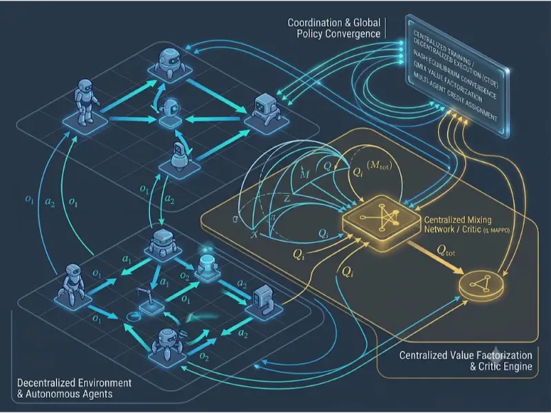
The key challenge in MARL is non-stationarity: because all agents update their decision policies in parallel, the environment’s state transition dynamics appear constantly changing from the perspective of any single agent. To address this non-stationarity, modern MARL frameworks utilize Centralized Training with Decentralized Execution (CTDE), Markov Games (Stochastic Games), and game-theoretic solution concepts such as the Nash Equilibrium to facilitate cooperative, competitive, or mixed coordination.
Interactive Quick Review: Non-Stationarity in Multi-Agent Environments
Why does treating a multi-agent environment as a collection of independent single-agent Q-learners fail to guarantee convergence?
Toggle Answer
Answer: Single-agent RL algorithms assume the environment transition probability P(s’ | s, a) is stationary. In multi-agent settings, transition dynamics depend on the joint action space of all agents. As other agents simultaneously update their policies, state transition probabilities shift over time, violating the Markov property and causing single-agent Q-values to oscillate or diverge.
Architectural & Theoretical Deep Dives
1. Markov Games (Stochastic Games) Formulation
A Markov Game with N agents is defined by the tuple (N, S, {Ai}i=1N, P, {Ri}i=1N, {Oi}i=1N, γ):
- State Space (S): The global environment state.
- Joint Action Space (A = A1 × A2 × … × AN): The set of combined actions chosen simultaneously by all N agents.
- Transition Probability (P(s’ | s, a)): The probability of transitioning from state s to s’ under joint action a.
- Reward Function (Ri(s, a)): Scalar reward awarded to agent i based on global state s and joint action a.
- Observation Function (Oi(s)): Partial observation tuple oi received by individual agent i in partially observable settings (POMDP).
2. Centralized Training with Decentralized Execution (CTDE)
CTDE balances global awareness during offline learning with autonomous execution during deployment:
- Centralized Training Phase: During training, a centralized critic module has access to extra information—such as global environment states s and joint actions a of all agents—to evaluate value functions accurately and stabilize credit assignment.
- Decentralized Execution Phase: At deployment, the centralized critic is removed. Each agent i selects its individual action ai strictly using its actor policy network πi(ai | oi), conditioned exclusively on its own local observation history.
3. Value Factorization Mechanics (VDN & QMIX)
In fully cooperative team settings sharing a global reward rtot, individual agent action choices must satisfy the Individual-Global-Max (IGM) principle:
$$\arg\max_{\mathbf{a}} Q_{\text{tot}}(s, \mathbf{a}) = \begin{pmatrix} \arg\max_{a_1} Q_1(o_1, a_1) \\ \vdots \\ \arg\max_{a_N} Q_N(o_N, a_N) \end{pmatrix}$$
Value Decomposition Networks (VDN) assume simple linear sum factorization: Qtot(s, a) = ∑ Qi(oi, ai).
QMIX generalizes this by passing individual utilities Qi into a non-linear Mixing Network conditioned on global state s. QMIX enforces the IGM condition by constraining the mixing network weights to be non-negative via absolute value projections:
$$\frac{\partial Q_{\text{tot}}(s, \mathbf{a})}{\partial Q_i(o_i, a_i)} \ge 0, \quad \forall i \in \{1, \dots, N\}$$
4. Python Implementation: Simplified QMIX Mixing Network
import torch

import torch.nn as nn

import torch.nn.functional as F


class QMIXMixingNetwork(nn.Module):

    """

    QMIX Mixing Network enforcing non-negative weights via absolute transformations

    to guarantee the Individual-Global-Max (IGM) condition.

    """

    def __init__(self, num_agents: int, state_dim: int, embed_dim: int = 32):

        super().__init__()

        self.num_agents = num_agents

        self.state_dim = state_dim

        self.embed_dim = embed_dim


        # Hypernetwork for Layer 1 weights and bias

        self.hyper_w1 = nn.Linear(state_dim, num_agents * embed_dim)

        self.hyper_b1 = nn.Linear(state_dim, embed_dim)


        # Hypernetwork for Layer 2 weights and bias

        self.hyper_w2 = nn.Linear(state_dim, embed_dim)

        self.hyper_b2 = nn.Sequential(

            nn.Linear(state_dim, embed_dim),

            nn.ReLU(),

            nn.Linear(embed_dim, 1)

        )


    def forward(self, agent_qs: torch.Tensor, states: torch.Tensor) -> torch.Tensor:

        """

        agent_qs: Individual agent Q-values [batch_size, 1, num_agents]

        states: Global environment state [batch_size, state_dim]

        """

        bs = agent_qs.size(0)


        # Layer 1: Generate non-negative weights via torch.abs()

        w1 = torch.abs(self.hyper_w1(states)).view(bs, self.num_agents, self.embed_dim)

        b1 = self.hyper_b1(states).view(bs, 1, self.embed_dim)

        hidden = F.elu(torch.bmm(agent_qs, w1) + b1)


        # Layer 2: Generate non-negative weights

        w2 = torch.abs(self.hyper_w2(states)).view(bs, self.embed_dim, 1)

        b2 = self.hyper_b2(states).view(bs, 1, 1)


        # Compute Q_tot

        q_tot = torch.bmm(hidden, w2) + b2

        return q_tot.view(bs, -1)


# Example Execution

batch_size = 4

num_agents = 3

state_dim = 16


mixer = QMIXMixingNetwork(num_agents=num_agents, state_dim=state_dim)

sample_q_vals = torch.tensor([[1.2, 0.5, 2.1], [0.8, 1.1, 0.4], [2.0, 1.8, 1.5], [0.1, 0.2, 0.3]]).unsqueeze(1)

sample_state = torch.randn(batch_size, state_dim)


q_tot_output = mixer(sample_q_vals, sample_state)

print("Output Joint Q_tot Shape:", q_tot_output.shape)

print("Calculated Q_tot Values:", q_tot_output.squeeze().detach().numpy())
Interactive Quick Review: Nash Equilibrium vs. Pareto Optimality
What is the key theoretical difference between a Nash Equilibrium and a Pareto Optimal joint policy in multi-agent game theory?
Toggle Answer
Answer: A Nash Equilibrium is a joint policy state where no individual agent can increase its personal expected reward by unilaterally changing its strategy, assuming all other agents keep their strategies fixed. A Pareto Optimal joint policy is an outcome where no agent’s reward can be strictly increased without making at least one other agent worse off.
Taxonomy & Optimization Comparison Matrix
| MARL Paradigm | Execution Mode | Coordination Type | Credit Assignment Strategy | Primary Advantage |
|---|---|---|---|---|
| Independent Q-Learning (IQL) | Decentralized | Competitive / Cooperative | None (Treats agents as environment) | Minimal memory footprint; highly scalable |
| MADDPG (Multi-Agent DDPG) | CTDE (Actor-Critic) | Mixed / Competitive | Centralized Critic with joint actions | Handles continuous multi-agent action spaces smoothly |
| QMIX | CTDE (Value-Based) | Fully Cooperative | Monotonic Mixing Hypernetwork | Guarantees exact decentralized max action selection |
| MAPPO (Multi-Agent PPO) | CTDE (Policy Gradient) | Cooperative / Mixed | Generalized Advantage Estimation (GAE) | High sample efficiency and empirical stability |
Applications, Trade-offs, & Future Outlook
Real-World Applications
- Autonomous Fleet Traffic Management: Coordinating self-driving ride-share fleets at city intersections without centralized traffic light signals.
- Smart Energy Microgrid Balancing: Distributed battery storage systems and solar nodes bidding power autonomously across decentralized smart grids.
- Swarm Robotics Search & Rescue: Decentralized drone swarms navigating GPS-denied environments using local RF communication links.
Engineering Trade-offs
The main trade-off in MARL involves Scalability vs. Coordination Efficiency. Fully centralized controllers eliminate non-stationarity but suffer from exponential state-action space explosion (|A|N), making them intractable for more than a few agents. Decentralized methods scale effortlessly but struggle with the Multi-Agent Credit Assignment Problem—disentangling which specific agent’s action contributed to team success or failure when receiving a shared global reward signal.
Future Outlook & Emerging Research
Frontier research centers on Mean Field Games (MFG)—which approximate infinite-agent systems by modeling swarm populations as continuous probability distributions—and Graph Neural Network (GNN) Communication Architectures, which allow dynamic agent networks to pass topological communication messages dynamically during runtime.
Frequently Asked Questions
What is the Multi-Agent Credit Assignment Problem?
In cooperative multi-agent tasks sharing a team reward, credit assignment is the challenge of identifying which specific agent actions contributed positively to the global outcome and which performed poorly, preventing “lazy agent” behaviors.
How does MAPPO differ from standard single-agent PPO?
MAPPO uses standard individual PPO policies for actors, but conditions the centralized Value Critic network on the global environment state (or joint agent observations and actions), providing variance-reduced baseline estimates during training.
Why can’t VDN handle complex cooperative tasks as effectively as QMIX?
VDN assumes that the global Q-value is simply the additive sum of individual Q-values (∑ Qi). This strict linear assumption cannot represent complex non-linear feature interactions between agents that QMIX captures using its hypernetwork-driven mixing architecture.
What is a Zero-Sum Markov Game?
A Zero-Sum Markov Game is a strictly competitive two-team environment where the sum of rewards across all agents equals zero (∑ Ri = 0), meaning one agent’s reward gain is directly equal to its opponent’s loss.
End-of-Page Exercises & Assessment
Part 1: Review Questions
Q1: Define Centralized Training with Decentralized Execution (CTDE).
Answer: CTDE is a paradigm where agents utilize global state information and joint actions during offline centralized training to stabilize learning, but rely exclusively on local observations during real-time decentralized execution.
Q2: State the Individual-Global-Max (IGM) condition.
Answer: The IGM condition asserts that a greedy action selection chosen individually across local agent utilities Qi(oi, ai) yields the exact same joint action as maximizing the global joint action-value function Qtot(s, a).
Q3: How does QMIX mathematically enforce the IGM condition?
Answer: QMIX enforces IGM by constraining all weight parameters of its central mixing network to be non-negative via absolute value transformations (∂Qtot / ∂Qi ≥ 0).
Q4: Why does environmental non-stationarity occur in Independent Q-Learning?
Answer: Because all agents adapt their action selection policies simultaneously, making state transition probabilities P(s’ | s, ai) continuously shift over time from the local perspective of agent i.
Q5: What is a Pure Strategy Nash Equilibrium?
Answer: A deterministic action combination a* = (a1*, …, aN*) where no individual agent i can improve its expected reward Ri(s, ai, a–i*) by unilaterally switching to a different action ai ≠ ai*.
Part 2: Thought-Provoking Questions
Q1: Communication Bottlenecks and Adversarial Jamming
Scenario: A swarm of 20 autonomous delivery drones operates in an environment where RF communication channels suffer from random packet loss and adversarial jamming.
Analysis: If agents rely on explicit communication bandwidth (passing continuous feature vectors to neighbors), network outages disrupt coordination policies, causing catastrophic failures. A robust MARL design should utilize Communication-Free CTDE (such as QMIX or MAPPO) where coordination strategies are internalized into local execution policies during offline training, enabling effective autonomous decision-making even during total communication blackout.
Q2: The Lazy Agent Problem in Cooperative Swarms
Scenario: During joint team training with a single shared reward, three agents actively perform the target task while a fourth agent sits idle to avoid incurring movement energy penalties.
Analysis: This is an example of the multi-agent credit assignment failure known as the “Lazy Agent Problem.” Because the team reward is positive, the passive agent receives positive reinforcement despite contributing nothing. Mitigating this requires counterfactual credit assignment methods (such as COMA) or marginal contribution value factorization (such as QMIX) that calculate an agent’s individual impact relative to a counterfactual baseline.
Part 3: Numerical Engineering Problems
Problem 1: 2×2 Matrix Game Nash Equilibrium & Dominant Strategies
Question: Consider a 2-agent cooperative game with payoff matrix for Agent 1 and Agent 2 given by joint rewards (R1, R2):
• Action (A, A): (4, 4)
• Action (A, B): (0, 2)
• Action (B, A): (2, 0)
• Action (B, B): (1, 1)
1. Determine if Agent 1 or Agent 2 has a strictly dominant action.
2. Identify all Pure Strategy Nash Equilibria (PSNE) of this game.
Step-by-step Solution:
1. Analyze Agent 1’s payoffs:
• If Agent 2 chooses A: Action A yields 4, Action B yields 2. (A is better: 4 > 2)
• If Agent 2 chooses B: Action A yields 0, Action B yields 1. (B is better: 1 > 0)
Since the optimal action depends on Agent 2’s choice, Agent 1 has no strictly dominant strategy.
2. Analyze Agent 2’s payoffs:
• If Agent 1 chooses A: Action A yields 4, Action B yields 2. (A is better: 4 > 2)
• If Agent 1 chooses B: Action A yields 0, Action B yields 1. (B is better: 1 > 0)
Agent 2 also has no strictly dominant strategy.
3. Test for Pure Strategy Nash Equilibria:
• Pair (A, A): Agent 1 shifting to B lowers payoff from 4 to 2. Agent 2 shifting to B lowers payoff from 4 to 2. Neither wants to deviate. → (A, A) is a Nash Equilibrium.
• Pair (B, B): Agent 1 shifting to A lowers payoff from 1 to 0. Agent 2 shifting to A lowers payoff from 1 to 0. Neither wants to deviate. → (B, B) is a Nash Equilibrium.
Final Answer: Neither agent has a dominant strategy. The game has two Pure Strategy Nash Equilibria at (A, A) with payoffs (4,4) and (B, B) with payoffs (1,1).
Problem 2: QMIX Monotonic Value Factorization Verification
Question: A 2-agent QMIX system has individual utility values Q1(o1, a1) = 2.0 and Q2(o2, a2) = 3.0. The mixing network computes global value Qtot using hypernetwork weights w1 = 0.5, w2 = 0.8, and bias b = 0.4 via linear mixing: $$Q_{\text{tot}} = w_1 Q_1 + w_2 Q_2 + b$$ 1. Calculate the initial Qtot. 2. If Agent 1 increases its local utility to Q1‘ = 3.5 while Agent 2 remains fixed, verify that the monotonicity condition ∂Qtot / ∂Q1 ≥ 0 holds by computing the new Qtot‘.
Step-by-step Solution:
1. Calculate initial Qtot: $$Q_{\text{tot}} = (0.5 \times 2.0) + (0.8 \times 3.0) + 0.4 = 1.0 + 2.4 + 0.4 = 3.8$$
2. Compute partial derivative ∂Qtot / ∂Q1:
∂Qtot / ∂Q1 = w1 = 0.5 ≥ 0
3. Compute updated Qtot‘ with Q1‘ = 3.5: $$Q_{\text{tot}}’ = (0.5 \times 3.5) + (0.8 \times 3.0) + 0.4 = 1.75 + 2.4 + 0.4 = 4.55$$
Final Answer: Initial Qtot = 3.8. The derivative ∂Qtot / ∂Q1 = 0.5 ≥ 0 confirms monotonicity, increasing the joint value to Qtot‘ = 4.55.
Reinforcement Learning Sub-Cluster
-
RLHF & AI Alignment
Explore PPO, DPO, reward modeling, and aligning foundation models with human utility and intent. -
Model-Based RL & Sim-to-Real Transfer
Master world models, dynamics prediction, domain randomization, and transferring policies to robotics. -
Reinforcement Learning Hub
Return to the main Reinforcement Learning overview covering MDPs, Q-Learning, Policy Gradients, and Actor-Critic methods.
External Academic & Technical References
- QMIX: Monotonic Value Function Factorisation for Deep Multi-Agent Reinforcement Learning (Rashid et al., ICML 2018) – Foundational paper on non-linear monotonic value factorization in cooperative MARL.
- Multi-Agent Actor-Critic for Mixed Cooperative-Competitive Environments (Lowe et al., MADDPG) – Key paper introducing centralized critic learning for continuous multi-agent environments.
- The Surprising Effectiveness of PPO in Cooperative Multi-Agent Games (Yu et al., MAPPO) – Comprehensive study demonstrating state-of-the-art multi-agent performance using PPO with centralized critics.