
Prepare for University Studies & Career Advancement

Stellar Atmospheres and Spectroscopy

The field of stellar atmospheres and spectroscopy models the physical processes of radiative transfer within the outer, optically thin layers of a self-gravitating plasma configuration. Because stellar interiors are completely inaccessible to direct empirical sampling, the electromagnetic flux escaping the photosphere provides the definitive source of quantitative data regarding a star’s macroscale properties. By applying quantum mechanics and thermodynamic boundary conditions to these radiative signatures, stellar physics translates starlight into explicit calculations of effective surface temperature, elemental abundance matrices, surface gravity, kinematics, and evolutionary status.
A stellar atmosphere is defined as the transition zone from which internal radiative energy finally decouples from the high-opacity stellar plasma and propagates into the vacuum of space. Although this layer constitutes a negligible fraction of the star’s total mass tensor, its structural architecture serves as the definitive boundary condition for all outward energy transport. As continuous blackbody radiation from the deeper layers diffuses through this cooler, lower-density atmosphere, specific gas ions, atoms, and molecules absorb and emit discrete photons at quantized energy levels, carving a complex network of absorption and emission lines into the continuous spectrum.
Spectroscopy is the analytical methodology used to disperse this escaping flux into its constituent monochromatic wavelengths. By matching the observed patterns of spectral lines against laboratory-validated quantum transitions, astrophysicists isolate the distinct quantum signatures of elements such as hydrogen, helium, calcium, sodium, and iron-peak metals. Furthermore, evaluating the widths, profiles, and shifts of these lines yields precise calculations of gas pressure, local plasma density, bulk fluid velocity fields, and magnetic flux densities, transforming distant points of light into rigorous physical records.
This diagnostic framework remains structurally linked to the core thermodynamic engines detailed in nuclear fusion in stellar physics, as the total energy flux produced by core tunneling kinetics sets the ultimate boundary conditions for atmospheric heating. It serves as the primary tool for mapping star life cycles, as a star’s position on the Hertzsprung-Russell diagram is determined explicitly by its spectral type and luminosity class. The heavy element metal yields forged via stellar nucleosynthesis leave indelible chemical markers in the absorption profiles, while tracking variations through variable stars and stellar oscillations maps the real-time hydrodynamic variations of the atmosphere.
Stellar spectroscopy provides the empirical foundations needed to decode the extreme physical parameters characterizing stellar remnants. Non-fusing compact structures like white dwarfs and neutron stars feature unique spectral modifications—such as extreme gravitational redshifts and severe pressure broadening—that allow physicists to validate Fermi degeneracy equations and track how matter behaves under gravitational and magnetic stresses unavailable in terrestrial laboratories.
For university-bound STEM students, the core principle is absolute: spectroscopy bridges quantum atomic transitions with macroscopic cosmic phenomena. It demonstrates how the integration of thermodynamics, statistical mechanics, and optics allows researchers to decode the exact material and kinematic evolution of systems situated thousands of light-years away. Learning to parse these radiative signatures transforms distant light into highly structured, verifiable physical data.
Stellar Spectroscopy: illustrating how light from a star is analyzed to reveal its composition and properties.
Key Invariant: The stellar atmosphere operates as the radiative boundary interface where internal energy thermalizes and decouples from plasma opacities, embedding quantum atomic signatures into the escaping flux that disclose the physical parameters of the star.

Analytical Reflection: Quantum Inversion of the Photospheric Flux

Analyze how atomic transitions within low-density gas layers encode structural data into continuous radiation paths.
If you cannot touch, visit, or collect a sample from a star, how can its light still reveal what the star is made of and how it is changing?
Analytical Prompt: Evaluate this by modeling how local thermodynamic equilibrium (LTE) dictates the source function, exploring the quantum mechanics of bound-bound absorption transitions, and tracking how Doppler velocity vectors shift spectral line centroids across cosmic distances.


Suggested Analytical Response: Starlight carries highly structured information due to the micro-physical interaction of photons with quantized atomic states within the stellar atmosphere:

1. Bound-Bound Quantum Transitions: Continuous blackbody radiation originating from the high-optical-depth layers must pass through the cooler, less dense gas of the upper photosphere. Photons with energies matching the exact difference between two electron orbitals ($\Delta E = h\nu$) are absorbed by local atoms and ions. When these excited states decay, the photons are re-emitted isotropically, creating a localized deficit of flux along the observer’s line of sight, manifesting as dark absorption lines that act as element-specific chemical fingerprints.

2. Thermodynamic State Calibration: The strength and ionization state of these spectral lines are governed by the local temperature and electron pressure grids, calculated quantitatively by coupling the Boltzmann and Saha ionization equations. This allows astrophysicists to invert the observed line ratios to determine the absolute effective temperature ($T_{\text{eff}}$) and surface gravity ($\log g$) of the plasma matrix.

3. Kinematic Vector Modulation: Macroscale physical modifications shift these line profiles. Bulk radial velocities compress or expand the wave vectors, driving measurable Doppler shifts ($\frac{\Delta \lambda}{\lambda_0} = \frac{v}{c}$) that reveal the star’s spatial motion and atmospheric oscillations, while high-velocity rotations or thermal gas motions broaden the line shapes to provide insights into stellar rotation and turbulence.

Key Invariant: Stellar spectroscopy reverses the absorption markers carved by quantized atomic states, transforming raw electromagnetic flux into empirical calculations of stellar composition, thermodynamics, and kinematics.

Light Emission and Observable Signatures

The field of stellar atmospheres and spectroscopy provides the definitive quantitative link between abstract theoretical physics and observational data. This navigation structure maps the integration of radiative spectral observations across the broader Stellar Physics curriculum, illustrating how the micro-physics of photon-matter interactions decodes thermodynamic profiles, core fusion kinetics, structural oscillations, and the boundaries of degenerate matter.

Stellar Physics Core Frameworks

Establishes the macroscale mathematical models of stellar interiors, defining how mechanical equilibrium and local thermodynamic state grids dictate the global radiative flux that eventually escapes through the atmospheric boundary layer.

Stellar Atmospheres and Spectroscopy

Investigates the micro-physical processes of radiative transfer, applying quantum atomic physics, absorption cross-sections, and line broadening tensors to invert escaping light into calculations of chemical abundances, kinematics, and surface gravities.

Variable Stars and Stellar Oscillations

Analyzes time-resolved spectral line profile variations and Doppler velocity displacements, using asteroseismic wave propagation to directly audit the hydrodynamic pulsations and internal structural reconfigurations of active stars.

Nuclear Fusion Mechanics

Links the emerging atmospheric bolometric flux back to its micro-physical source: the subatomic quantum tunneling kinetics and core temperature-sensitive reaction networks that produce the primary energy driving stellar engines.

Stellar Nucleosynthesis Networks

Decodes the elemental abundance traces embedded as absorption features within the photosphere, providing empirical evidence of the successive alpha-capture chains and neutron-capture tracks that alter cosmic matter.

Star Life Cycles

Tracks the historical evolution of stellar spectra across the Hertzsprung-Russell diagram, evaluating how a system’s atmospheric parameters, mass-loss wind opacities, and molecular line tracers shift as it moves from protostellar birth to terminal states.

Stellar Remnants: Neutron Stars and White Dwarfs

Examines the highly modified spectral properties of non-fusing compact remnants, using extreme pressure broadening, molecular Zeeman splittings, and gravitational redshifts to validate equations of state under ultra-dense regimes.
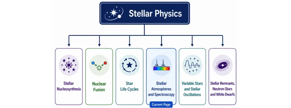
Structure chart showing Stellar Physics as the parent page connected to Stellar Nucleosynthesis, Nuclear Fusion, Star Life Cycles, Stellar Atmospheres and Spectroscopy, Variable Stars and Stellar Oscillations, and Stellar Remnants Neutron Stars and White Dwarfs, with Stellar Atmospheres and Spectroscopy marked as the current page.
A structure chart showing Stellar Atmospheres and Spectroscopy as the current page within the wider Stellar Physics cluster.
This structure chart presents Stellar Physics as the parent topic and shows its related child pages: Stellar Nucleosynthesis, Nuclear Fusion, Star Life Cycles, Stellar Atmospheres and Spectroscopy, Variable Stars and Stellar Oscillations, and Stellar Remnants Neutron Stars and White Dwarfs. Stellar Atmospheres and Spectroscopy is highlighted as the current page, helping students understand how the study of stellar light, spectra, composition, temperature, and atmospheric layers fits within the broader Stellar Physics cluster.

Structure of Stellar Atmospheres

A stellar atmosphere is not modeled as a single homogeneous gas shell. Instead, it is structured as a series of stratified, concentric envelopes, each characterized by distinct thermodynamic gradients, localized plasma opacities, magnetohydrodynamic (MHD) velocity fields, and unique radiation signatures. These layers dictate the optical depth parameters that shape the electromagnetic flux emerging from the star.
For main-sequence stars like the Sun, this coupled architecture is divided into three primary functional zones: the photosphere, the chromosphere, and the corona. Analyzing these domains allows physicists to mathematically solve the equations of radiative transfer, evaluate atmospheric boundary heating mechanisms, and map the magnetic field interactions that drive stellar activity into the surrounding space environment.

The Photosphere

The photosphere represents the primary visible boundary layer of a star, defined mathematically as the region where the optical depth (\(\tau_\lambda\)) across visible wavelengths drops to approximately \(\tau \approx 2/3\). Below this boundary, the plasma matrix is opaque; at this interface, the mean free path of photons approaches infinity, allowing radiation to decouple from the fluid and escape into space.
For a solar-mass engine, the photosphere exhibits an effective temperature (\(T_{\text{eff}}\)) of approximately \(5{,}778\,\text{K}\). According to Wien’s displacement law (\(\lambda_{\text{max}} T = b\)), this thermal baseline causes the continuous blackbody spectrum to peak in the visible band. Variations in mass allocation shift this temperature constraint: high-mass stars exhibit elevated temperatures that shift their emission profiles into the ultraviolet, while low-mass configurations radiate predominantly in the red and infrared spectrums.
The cooler upper boundaries of the photosphere are responsible for carving <strong>Fraunhofer absorption lines</strong> into the continuous flux. Continuous blackbody radiation from deeper, high-optical-depth layers passes through the less dense, cooler gas layers above. Localized atoms and ions undergo bound-bound quantum transitions, absorbing discrete photon wavelengths. This process creates a net deficit of flux along the observer’s line of sight, mapping the exact chemical element composition of the plasma.
Mechanically, the photosphere marks the upper boundary of the convective zone, displaying a highly dynamic <strong>granulation</strong> pattern. These granules represent the top of gas buoyancy columns where hot, low-density plasma cells rise at velocities of \(v \approx 1 \rightarrow 2\,\text{km/s}\), radiate their thermal energy at the optical surface, increase in density, and sink back down along cooler, dark intergranular lanes. This fluid circulation acts as the primary mechanism for convective energy transport immediately prior to radiative decoupling.

The Chromosphere

Situated immediately above the photospheric boundary is the chromosphere, a lower-density layer extending roughly \(2{,}000\,\text{km}\) radially. Within this domain, the temperature profile stops declining and reverses, establishing a positive temperature gradient where temperatures rise with altitude from a minimum of \(T \approx 4{,}200\,\text{K}\) up to \(T \approx 25{,}000\,\text{K}\). This thermal inversion violates classical thermodynamic cooling models and is driven by mechanical energy dissipation from acoustic waves and magnetohydrodynamic Alfvén waves generated by the underlying convection zone.
During solar eclipses, the chromosphere manifests visually as a faint reddish flash, an optical signature driven by intense quantum emission from the hydrogen-alpha (\(\text{H}\alpha\)) transition line at \(\lambda = 656.3\,\text{nm}\). This layer serves as an essential laboratory for analyzing non-local thermodynamic equilibrium (non-LTE) physics, where radiation fields are decoupled from the local kinetic temperature matrix.
The chromosphere features highly dynamic plasma jets known as spicules—supersonic gas columns that project upward into the lower corona at velocities exceeding \(v \approx 20\,\text{km/s}\) before collapsing. These structural features act as mass transport channels, channeling ionized gas and magnetic flux upward into the extended stellar atmosphere.
Because the upper chromosphere consists of hot, partly ionized gas, it produces distinct <strong>emission lines</strong> across ultraviolet wavelengths. Evaluating the intensity ratios of these emission profiles allows astronomers to calculate the non-thermal heating coefficients, magnetic field strengths, and flash energy generation rates that govern stellar activity.

The Corona

The corona constitutes the outermost, highly extended envelope of the stellar atmosphere, expanding across millions of kilometers into space where it transitions into the kinetic acceleration zone of the solar wind. Although characterized by an exceptionally low particle density (\(n \approx 10^8\,\text{cm}^{-3}\) near the base), the corona features an extreme thermal inversion, with temperatures soaring to \(T \approx 1 \rightarrow 3 \times 10^6\,\text{K}\).
This anomalous coronal heating remains a primary focus of modern astrophysics. Because the underlying photosphere is several orders of magnitude cooler, heat cannot be transferred via traditional thermal conduction. Instead, energy is pumped into the corona via magnetic mechanisms, including <strong>magnetic reconnection</strong> loops—where twisted magnetic field lines snap and release stored energy—and high-frequency Alfvén wave dissipation within open magnetic field regions.
Due to these extreme temperatures, the coronal plasma is highly ionized (e.g., stripping iron down to \(\text{Fe}^{13+}\)) and emits strongly in high-energy X-ray and extreme ultraviolet (EUV) channels according to the Stefan-Boltzmann equation. Capturing these high-energy flux channels allows researchers to map magnetic coronal loops, track stellar flare dynamics, and model the magnetohydrodynamics of <strong>coronal mass ejections (CMEs)</strong>.
While visible to the naked eye only as a white halo during total eclipses due to Thomson scattering of photospheric light by free electrons, the corona’s primary physical significance lies in its role as a particle accelerator. The high thermal pressure overrides the star’s local gravitational potential, driving a continuous hydrodynamic expansion that shapes space weather profiles and modulates planetary magnetospheres throughout the stellar system.
Key Invariant: The stellar atmosphere is organized into a three-tiered thermodynamic architecture: the photosphere drives radiative decoupling and absorption lines; the chromosphere marks the onset of magnetic thermal inversion; and the corona accelerates ultra-hot, low-density plasma into interstellar space.

Analytical Reflection: Decoupling the Layer Signatures

Analyze how specific layer parameters map unique quantum and high-energy markers into the aggregate spectral flux.
A spectrum shows dark absorption lines from cooler gases, a reddish emission glow above the visible surface, and high-energy X-ray emission from very hot thin plasma. Which atmospheric layers are mainly responsible for these three signatures?
Analytical Prompt: Evaluate this by tracking optical depth boundaries (\(\tau = 2/3\)) for absorption mechanics, modeling bound-bound Balmer series emission constraints, and applying the plasma ionization equations that govern high-energy bremsstrahlung radiation.


Suggested Analytical Response: The distinct spectral profiles are direct products of the stratified atmospheric layers:

1. Photospheric Absorption: The dark absorption lines are carved at the optical depth interface (\(\tau \approx 2/3\)) of the photosphere, where the escaping continuous blackbody flux passes through cooler, low-pressure gas, driving bound-bound quantum absorption states.

2. Chromospheric Emission: The reddish glow originates within the chromosphere, where non-LTE conditions and mechanical heating elevate gas temperatures enough to populate the \(n=3\) state of hydrogen, driving a high-frequency \(\text{H}\alpha\) (\(3 \rightarrow 2\)) Balmer emission channel.

3. Coronal High-Energy Flux: The X-ray emission is generated deep within the corona, where magnetic reconnection loops pump temperatures past \(T \ge 10^6\,\text{K}\). This high thermal energy strips valence electrons from heavy metals, generating high-energy bremsstrahlung and characteristic X-ray line emissions from highly ionized atomic states.

Key Invariant: Isolating individual wavelength bands isolates the specific atmospheric layers, allowing for the independent calculation of a star’s photospheric chemistry, chromospheric waves, and coronal magnetism.

Spectral Analysis and Stellar Spectroscopy

Spectroscopy is the core analytical methodology used to disperse continuous starlight into its constituent monochromatic wavelengths. Rather than observing a star as a single unresolved point source, spectroscopy permits the precise mapping of radiation density distributions over discrete frequency bounds. By measuring the absolute intensity profiles, continuum colors, absorption lines, emission lines, and wavelength centroids, physicists resolve the absolute state metrics of distant stellar atmospheres.

Spectral Lines

Spectral lines represent the localized absorption or emission features carved into a continuous spectrum by bound-bound quantum electronic transitions. The exact wavelength (\(\lambda\)) of each line is governed by the Planck-Einstein relation (\(\Delta E = \frac{hc}{\lambda}\)), matching the discrete energy differences between localized electron orbitals within specialized atomic configurations.
Absorption lines manifest as localized reductions in the continuous radiation field. They are generated when continuous blackbody radiation originating from high-optical-depth core layers propagates through outer, lower-temperature atmospheric envelopes. Incoming photons with energy states matching local quantum transitions are absorbed, driving bound electrons to elevated excitation levels. These electrons subsequently decay via isotropic photon re-emission, creating a net line-of-sight flux deficit along the observer’s line of sight.
Emission lines manifest as narrow channels of intense radiative flux. They form when low-density, highly energized gas undergoes spontaneous radiative de-excitation, emitting photons along specific line-of-sight paths. These markers serve as structural diagnostics for low-density, high-temperature domains such as stellar chromospheres, extended stellar envelopes, planetary nebulae shells, and shock-heated circumstellar active regions.

Doppler Effect and Radial Velocity Kinetics

The Doppler effect modulates the observed wave vector of starlight when a stellar system possesses a non-zero velocity component relative to the observer. If a star exhibits motion directed away from Earth, the observed wave vectors are stretched toward longer, lower-frequency wavelengths—a phenomenon designated as redshift. Conversely, if the system moves toward the observer, the wave vectors are compressed toward shorter, higher-frequency paths, yielding a blueshift.
By measuring the exact shift of a spectral line centroid (\(\Delta \lambda\)) relative to its laboratory rest frame (\(\lambda_0\)), physicists compute the system’s exact radial velocity (\(v_r\)):
\[\frac{\Delta \lambda}{\lambda_0} = \frac{v_r}{c}\]
This kinematic tool allows for the calculation of orbital elements in spectroscopic binary configurations, the profiling of stellar rotation vectors via line profile broadening, and the calculation of galactic expansion rates.
This precision tracking provides the empirical framework for detecting exoplanetary systems via the radial velocity technique. As an exoplanet orbits its host star, their mutual orbit around the system’s common center of mass induces a periodic mechanical toggle in the star’s velocity vector. The resulting periodic red-blue shifting of the star’s photospheric absorption lines enables the calculation of the planet’s orbital period and lower mass boundaries (\(M \sin i\)).

The Zeeman Effect

The Zeeman effect models the splitting of degenerate atomic energy states in the presence of an external magnetic field (\(B\)). Under standard quantum mechanics, orbital angular momentum states possess degenerate energy boundaries; introducing a powerful magnetic field breaks this spatial degeneracy by interacting with the electron’s magnetic dipole moment, splitting the single atomic state into multiple discrete, polarized energy levels.
Astrophysicists analyze this splitting to map the magnetohydrodynamic (MHD) architectures of stellar atmospheres. Measuring the magnitude of the line separation (\(\Delta \lambda_Z\)) provides a direct quantitative probe of magnetic flux densities within sunspots, starspots, active flare regions, and the global convective dynamos of highly magnetized stars:
\[\Delta \lambda_Z \propto g_{\text{eff}} \lambda^2 B\]
Key Invariant: Stellar spectroscopy reverses the macroscale and subatomic modifications embedded within escaping starlight: electronic transitions index chemical species, Doppler shifts quantify radial kinematics, and Zeeman splitting tracks magnetic field tensors.

Quick Check: Decoding the Integrated Spectrum

Use this prompt to connect common spectral signatures with the physical information they reveal.
A star’s spectrum shows dark absorption lines, a repeated red-blue shifting of those lines, and slight splitting of some spectral lines. What can astronomers infer from these three clues?
Analytical Prompt: Evaluate this by tracking optical depth absorption limits, applying the Doppler velocity vector equation, and calculating the quantum mechanical effects of broke degeneracy via the Zeeman relation.
Suggested Analytical Response: The three distinct observations isolate independent physical conditions:

1. Fraunhofer Absorption lines: Prove the presence of specific atomic or ionic species inside the cooler layers of the photosphere, where incoming photons match bound-bound electronic excitation paths.

2. Periodic Doppler Shifts: Indicate that the star possesses a variable radial velocity vector, revealing center-of-mass orbital motion driven by a binary stellar companion or an orbiting exoplanet.

3. Refined Zeeman Component Splitting: Confirms the presence of intense magnetic fields breaking the quantum degeneracy of electron energy states, allowing for the direct calculation of localized magnetic flux tensors.
Key Invariant: The aggregate spectrum contains superimposed quantum, kinematic, and magnetic signatures that can be mathematically separated to map the state of the stellar atmosphere.

Chemical Composition Analysis

Chemical composition analysis converts the relative strengths and profiles of photospheric absorption lines into explicit calculations of elemental abundances within the stellar atmosphere. Because each element features a unique distribution of quantized electronic states, the resulting absorption line networks act as unique chemical signatures, enabling precise chemical abundance mapping across cosmic distances.
For example, hydrogen transitions originating from the \(n=2\) state yield the highly diagnostic Balmer series across visible wavelengths (e.g., \(\text{H}\alpha\) at \(656.3\,\text{nm}\), \(\text{H}\beta\) at \(486.1\,\text{nm}\)), acting as primary structural anchors in hot stars. Concurrently, specialized transitions from neutral and ionized helium (\(\text{He I}\), \(\text{He II}\)), ionized calcium (\(\text{Ca II}\) H and K lines), neutral sodium (\(\text{Na I}\) D lines), and complex neutral iron (\(\text{Fe I}\)) grids allow physicists to profile the entire elemental chemistry of the atmospheric plasma.
However, translating line strength directly into mass abundance requires solving complex thermodynamic state equations. The absolute equivalent width (\(W_\lambda\)) of an absorption line does not scale linearly with elemental density alone; rather, it is heavily modulated by the local plasma temperature, electron pressure grids, and the ionization balance defined by the Boltzmann and Saha equations. A weak spectral line does not imply element scarcity; it typically proves that the atmospheric temperature profile is unfavorable for populating that specific electronic level.
Within cooler stellar configurations (\(T_{\text{eff}} \le 4{,}000\,\text{K}\)), low kinetic energies permit the formation of stable molecular bonds within the upper atmosphere. Complex molecular absorption bands—such as titanium oxide (\(\text{TiO}\)), carbon monoxide (\(\text{CO}\)), and cyanogen (\(\text{CN}\))—emerge in the spectra of late-type stars. These molecular bands introduce dense networks of closely spaced absorption lines that increase the global opacity profile of the stellar atmosphere.
Calculating these chemical parameters allows physicists to reconstruct the chemical evolution history of the galaxy. A star’s atmospheric metallicity index (\([\text{Fe}/\text{H}]\)) provides a historical record of its birth environment. High-metallicity stars reveal that their parent molecular nebula had already been enriched by successive rounds of alpha-capture nucleosynthesis and Type II supernova explosions from earlier generations of high-mass stars, directly tracking the chemical enrichment history of the cosmos.
Key Invariant: Chemical composition analysis requires the simultaneous calibration of line strengths alongside thermodynamic ionization balances to isolate absolute elemental abundances from temperature-driven line variations.

Analytical Reflection: The Ionization Balance Paradox

Analyze how line variations reveal the underlying competition between thermal excitation and chemical abundance.
If two stars both show hydrogen lines, but one also shows strong metal lines and molecular bands, what might this suggest about their temperature, composition, or evolutionary history?
Analytical Prompt: Model this by tracking how low thermal kinetic energies permit molecular binding states, evaluating how temperature dictates the Boltzmann state population index, and parsing the relationship between stellar metallicity and cosmic enrichment.
Suggested Analytical Response: The presence of strong metal lines and molecular bands alongside hydrogen features reveals distinct structural and historical differences between the two systems:

1. Thermodynamic Phase Modulation: The appearance of molecular bands (such as \(\text{TiO}\)) proves that the second star features a significantly lower effective surface temperature (\(T_{\text{eff}} \le 3{,}800\,\text{K}\)). In high-temperature atmospheres, intense kinetic impacts break molecular bonds; cool atmospheres permit these bonds to persist, allowing complex vibrational and rotational transitions to absorb light.

2. Excitation Mechanics: The variation in metal lines is heavily driven by the temperature-dependent Boltzmann distribution. In cool stars, neutral iron (\(\text{Fe I}\)) and low-ionization states dominate because the thermal energy is insufficient to strip valence electrons, driving strong low-excitation lines despite identical underlying abundances.

3. Evolutionary Metallicity Fingerprinting: If a rigorous thermodynamic inversion proves that the metal line disparity persists after correcting for temperature, it marks a fundamental difference in metallicity (\([\text{Fe}/\text{H}]\)). The metal-rich star belongs to a younger cosmic generation formed from an interstellar medium highly enriched by earlier supernova nucleosynthesis events, whereas the metal-poor star tracks the pristine chemical signatures of an older cosmic epoch.
Key Invariant: The presence of molecular line states isolates cool atmospheric boundaries, while the calculated ratio of metal-to-hydrogen lines maps the historical chemical enrichment of the star’s birth environment.

Spectral Classification and Thermodynamic Diagnostics

Stellar classification models the multi-variable thermodynamic states of stellar atmospheres by parsing the diagnostic structural signatures embedded within photospheric absorption spectra. A star’s classification code does not simply categorize it; it maps the direct mathematical solution to the equations of local thermodynamic equilibrium (LTE). By tracking the specific state of ionization and excitation within the plasma matrix, classification yields precise empirical metrics for a star’s effective surface temperature (\(T_{\text{eff}}\)), surface gravity (\(\log g\)), absolute bolometric luminosity, and current evolutionary status.
The ultimate utility of this taxonomy lies in its ability to isolate absolute physical tensors from raw observational flux. By coupling spectral class directly with luminosity boundaries, astrophysicists establish a star’s exact coordinates across the Hertzsprung-Russell diagram, breaking degeneracies between temperature and radius to reconstruct the past and future lifecycle of the stellar engine.

The Harvard Spectral Classification Framework

The Harvard spectral classification system structures stellar architectures along a continuous, monotonic effective surface temperature sequence, shifting from the hottest, high-mass configurations down to the coolest, low-mass objects:
\[O \rightarrow B \rightarrow A \rightarrow F \rightarrow G \rightarrow K \rightarrow M\]
This non-alphabetical sequence reflects a historical re-ordering of early line strength catalogs, restructured once the underlying quantum mechanics proved that line variation is driven by thermal excitation rather than discrete chemistry differences. Each spectral class is further divided into ten decimal subclasses (0 to 9) to map minor temperature increments (e.g., an O0 star represents the absolute thermal maximum of the O-type domain, while O9 bridges directly into B0).
Spectral ClassEffective Temperature (\(T_{\text{eff}}\), K)Continuum ColorDominant Quantum Spectral Features
O\(30{,}000 \rightarrow 50{,}000\)BlueSingly ionized helium (\(\text{He II}\)) absorption; highly ionized nitrogen and oxygen; exceptionally weak neutral hydrogen (\(\text{H I}\)) Balmer profiles.
B\(10{,}000 \rightarrow 30{,}000\)Blue-WhiteNeutral helium (\(\text{He I}\)) features achieve peak equivalent widths; neutral hydrogen lines scale from moderate to highly pronounced intensity profiles.
A\(7{,}500 \rightarrow 10{,}000\)WhiteNeutral hydrogen Balmer series (\(\text{H I}\)) achieve maximum absolute equivalent widths; singly ionized metals (\(\text{Mg II}\), \(\text{Si II}\)) begin to emerge.
F\(6{,}000 \rightarrow 7{,}500\)Yellow-WhiteHydrogen lines undergo rapid weakening; singly ionized calcium (\(\text{Ca II}\) H and K lines) and neutral metal profiles become highly prominent.
G\(5{,}200 \rightarrow 6{,}000\)YellowDominant \(\text{Ca II}\) H and K absorption; neutral metal lines (\(\text{Fe I}\), \(\text{Cr I}\)) dominate the opacity; hydrogen Balmer features are heavily suppressed.
K\(3{,}700 \rightarrow 5{,}200\)OrangeIntense neutral metal line networks dominate the entire optical spectrum; molecular bands (such as the \(\text{CH}\) G-band) initiate visible absorption trends.
M\(2{,}400 \rightarrow 3{,}700\)RedComplex molecular absorption bands—predominantly titanium oxide (\(\text{TiO}\))—cause severe continuum line blanketing; neutral metal lines remain deep.
The micro-physical mechanism driving this structural transition is governed by the Saha-Boltzmann Ionization Balance. Line strengths vary across classes not because of elemental abundance shifts, but because the atmospheric temperature profile dictates the exact quantum mechanical probability of an electron occupying a specific excitation and ionization tier. In hot O-stars, the kinetic energy is so extreme that hydrogen is fully ionized (\(\text{H}^+\)), leaving no bound electrons to generate Balmer lines; in cool M-stars, the low thermal velocity permits molecular binding states to persist, generating dense molecular absorption bands.

The Morgan-Keenan (MK) Luminosity Classification

Effective surface temperature alone cannot uniquely resolve a star’s structural parameters. Two distinct stars can share an identical effective temperature while exhibiting massive variations in physical radius, bolometric power output, and evolutionary path. For instance, an intermediate main-sequence star and an evolved supergiant can display identical colors while their absolute luminosities diverge by multiple orders of magnitude.
To resolve this degeneracy, astrophysicists deploy the Morgan-Keenan (MK) Luminosity Classification System. This taxonomy evaluates secondary spectral markers—specifically pressure broadening line widths—to calculate the star’s local surface gravity (\(\log g\)) and absolute size parameters. High-radius giant stars possess extended, low-density atmospheres that minimize particle collision frequencies, yielding exceptionally narrow absorption line profiles. Conversely, high-density main-sequence stars subject their atmospheric gas to intense pressure fields, driving severe collisional Stark broadening that expands the equivalent width of the line wings.
Luminosity ClassAstrophysical Structural ProfileEmpirical Representative Baseline
I (Ia / Ib)Supergiants: Extended, ultra-low density envelopes; minimal surface gravity indices (\(\log g \approx 0 \rightarrow 1\)); exceptionally sharp line widths.Betelgeuse (M1 Ia)
Rigel (B8 Ia)
IIBright Giants: Intermediate post-main-sequence structural reconfigurations bridging the giant and supergiant domains.Canopus (A9 II)
IIIGiants: Evolved post-main-sequence systems actively undergoing core helium or shell hydrogen burning stages.Aldebaran (K5 III)
IVSubgiants: Core hydrogen depleted; transitioning off the main sequence along Kelvin-Helmholtz thermal expansion tracks.Gamma Cephei (K1 IV)
VMain-Sequence Stars: Dense, steady-state core hydrogen-fusing dwarf configurations maintaining stable hydrostatic equilibrium.The Sun (G2 V)
VISubdwarfs: Metal-poor Population II stars exhibiting lower opacities that displace them below the standard main-sequence baseline.Kapteyn’s Star (sdM1)
VIIWhite Dwarfs: Compact, non-fusing, electron-degenerate remnants displaying extreme collisional Stark broadening signatures.Sirius B (DA2)
A comprehensive stellar classification expression synthesizes both the temperature subclass and the luminosity class into a singular code. For example, calibrating the solar spectrum yields a designation of G2 V. This configuration proves that the Sun is a yellow dwarf star situated at a temperature midpoint of \(T_{\text{eff}} \approx 5778\,\text{K}\) (indexed by G2), and actively resides within luminosity class V, proving that it maintains main-sequence hydrostatic balance via core hydrogen-to-helium fusion chains.
Key Invariant: The Harvard sequence dictates the effective surface temperature metric based on atomic ionization balances, while the Morgan-Keenan class determines the star’s physical radius and evolutionary phase via pressure broadening line diagnostics.

Quick Check: Decoding a Stellar Classification Code

Use this diagnostic prompt to audit your ability to invert a stellar classification expression into explicit physical parameters.
The Sun is classified as G2 V. What does this tell us about the Sun?
Analytical Prompt: Separate the quantitative thermodynamic implications of the G2 temperature subclass from the hydrodynamical and surface gravity indicators mapped by the V luminosity class.
Suggested Analytical Response: The composite classification code G2 V contains precise structural and thermodynamic state calculations:

1. Thermodynamic Core Calibration (G2): The G2 subclass anchors the star’s effective surface temperature at \(T_{\text{eff}} \approx 5778\,\text{K}\). At this thermal threshold, the gas kinetic energy favors neutral metal absorption lines—specifically neutral iron (\(\text{Fe I}\)) and singly ionized calcium (\(\text{Ca II}\)) K lines—while the thermal velocity is too low to maintain the hydrogen Balmer line strengths observed in hotter A-type stars.

2. Hydrodynamic Enclosure Profile (V): The Roman numeral V designates a main-sequence dwarf configuration. This proves that the star features a high surface gravity (\(\log g \approx 4.44\,\text{cgs}\)), which drives elevated particle collision frequencies within the photosphere, generating pronounced Stark line wing broadening. Mechanically, it proves that the core remains locked in long-term hydrostatic equilibrium sustained by core hydrogen fusion.
Key Invariant: A star’s full MK classification defines its exact position on the H-R diagram, binding its atmospheric temperature profile directly to its mechanical radius and core energy source.

Applications of Stellar Spectroscopy

Stellar spectroscopy operates as the primary quantitative diagnostic tool in nuclear astrophysics, allowing researchers to invert the electromagnetic signatures escaping the photosphere into explicit physical models of stellar interiors. Rather than treating a star as an isolated point source, spectroscopy permits the precise tracking of thermodynamic variables, subatomic reaction markers, kinematic velocity tensors, and localized magnetic fields across cosmic distances.

Determining Stellar Properties

A star’s spectrum provides the fundamental boundary parameters required to solve the equations of stellar structure. The effective surface temperature (\(T_{\text{eff}}\)) is constrained by fitting the continuum profile alongside the equivalent widths of key diagnostic absorption features. Furthermore, the absolute chemical composition (metallicity index \([\text{Fe}/\text{H}]\)) is calculated by measuring line intensities, which serve as direct empirical evidence of the alpha-capture chains and neutron-capture tracks operating inside the star.
Kinematic tensors are isolated by tracking line profile perturbations. The star’s radial velocity (\(v_r\)) is computed by measuring the displacement of spectral line centroids relative to their laboratory rest frames via the Doppler relation (\(\frac{\Delta \lambda}{\lambda_0} = \frac{v_r}{c}\)). Concurrently, the equatorial rotational velocity (\(v \sin i\)) is derived by evaluating rotational line broadening. As the star rotates, one hemisphere exhibits a localized blueshift while the opposite hemisphere undergoes a corresponding redshift; integrating this velocity gradient across the stellar disk translates the sharp quantum line profile into a broad, symmetrical absorption profile.

Studying Stellar Activity and Magnetohydrodynamics

Stellar atmospheres are dynamic fluid engines driven by complex magnetohydrodynamic (MHD) dynamos. Spectroscopy allows for the direct measurement of these magnetic fields by exploiting the Zeeman effect. When an atom undergoes an electronic transition within an intense magnetic field (\(B\)), the breaking of quantum spatial degeneracy splits individual absorption lines into polarized components, with the separation width (\(\Delta \lambda_Z \propto g_{\text{eff}} \lambda^2 B\)) providing a direct measurement of localized magnetic flux densities.
Furthermore, highly energetic events like stellar flares and active spot regions are tracked via time-resolved spectroscopy. During a flare event, rapid magnetic reconnection loops accelerate particles into the lower atmosphere, driving intense non-local thermodynamic equilibrium (non-LTE) shock heating. This changes the standard absorption profile into pronounced emission lines—specifically within the hydrogen-alpha (\(\text{H}\alpha\)) and ionized calcium (\(\text{Ca II}\) H & K) channels—allowing physicists to quantify the non-thermal energy dissipation rates that govern space weather dynamics.

Stellar Evolution and Lifecycle Tracking

A star’s spectrum acts as a real-time log of its position along its evolutionary track. Main-sequence dwarfs are distinguished by intense pressure broadening features (collisional Stark broadening) in their line wings due to high atmospheric densities (\(\log g \approx 4 \rightarrow 4.5\)). As the core exhausts its hydrogen and contracts, the star transitions into the red giant or supergiant domain; the resulting radial expansion reduces the atmospheric density and surface gravity (\(\log g \le 1\)), narrowing the spectral line profiles. Cooler giant envelopes also allow stable chemical bonds to form, introducing complex molecular bands (e.g., \(\text{TiO}\), \(\text{ZrO}\)) that signature late-stage stellar lifecycles.

Exoplanet Detection and Atmospheric Characterization

Stellar spectroscopy drives the discovery and analysis of extrasolar planetary systems through two primary methodologies:
  • The Radial Velocity Method: By measuring periodic, high-precision Doppler shifts in a star’s photospheric absorption lines, physicists detect the gravitational wobble induced by an orbiting exoplanet. This periodic modulation isolates the planet’s orbital period, eccentricity, and lower mass boundary (\(M \sin i\)).
  • Transit Transmission Spectroscopy: When an exoplanet passes directly in front of the stellar disk, a fraction of the photospheric flux filters through the planet’s thin atmospheric envelope. By subtracting the out-of-transit stellar spectrum from the in-transit spectrum, astronomers isolate the minute absorption signatures carved by the planet’s atmosphere, identifying chemical species such as water vapor (\(\text{H}_2\text{O}\)), carbon dioxide (\(\text{CO}_2\)), methane (\(\text{CH}_4\)), and vaporized metals.
Key Invariant: Stellar spectroscopy decodes superimposed atomic, kinematic, and magnetic signals from starlight, transforming raw observational flux into precise measurements of stellar physics and exoplanetary chemistry.

Analytical Reflection: Deconstructing Multi-Layered Spectral Signals

Analyze how concurrent physical processes embed distinct geometric and quantum modifications into a single spectral line profile.
A star’s spectrum shows strong hydrogen lines, a small repeating Doppler shift, broadened absorption lines, and occasional emission changes during flares. What different things can astronomers learn from these clues?
Analytical Prompt: Evaluate this by modeling how ionization states reflect temperature, how center-of-mass orbital mechanics govern radial velocity vectors, and how convective dynamos drive fluid line-broadening profiles.
Suggested Analytical Response: The individual spectral markers reveal distinct physical properties:

1. Hydrogen Balmer Equivalence Widths: Constrain the star’s effective surface temperature (\(T_{\text{eff}}\)), as the strength of these transitions maps the exact thermal kinetic energy required to populate the \(n=2\) atomic state without driving complete ionization.

2. Periodic Line Centroid Shifts: Unveil a variable radial velocity vector, providing direct mathematical evidence of a companion object—such as an exoplanet or a brown dwarf—exerting a gravitational pull around a mutual center of mass.

3. Symmetrical Profile Broadening: Quantifies the stellar rotation vector (\(v \sin i\)) through the integration of blue-shifted and red-shifted Doppler components across the rotating stellar hemispheres.

4. Transient Emission Flux: Signals sudden magnetohydrodynamic adjustments in the upper atmosphere, where magnetic reconnection loops release stored energy to heat the local plasma, driving spontaneous de-excitation emission.
Key Invariant: A single stellar spectrum contains a superimposed record of the star’s thermal structure, orbital motion, rotation rate, and magnetic field variations.

Advancements in Spectroscopic Technology

Modern stellar spectroscopy has advanced far beyond simply resolving visible light into colors. Today, astrophysicists deploy high-precision, fiber-fed instruments, space-based telescopes, and multi-wavelength echelle spectrographs to capture faint spectral transitions, micro-Doppler velocity variations, non-thermal magnetic loops, and atmospheric signatures with extreme sub-angstrom precision.
These technological leaps allow scientists to map the fine structural dynamics of stellar interiors, discover low-mass exoplanetary architectures via indirect gravitational diagnostics, model non-LTE atmospheric boundaries, and observe physical high-energy systems hidden from ground-based view.

High-Resolution Echelle Spectrographs

High-resolution spectrographs (\(R = \frac{\lambda}{\Delta \lambda} \ge 100{,}000\)) utilize crossed dispersion gratings to separate starlight into incredibly fine wavelength steps. This allows astronomers to detect microscale shifts, profile broadening, and asymmetric line splittings that disclose atmospheric turbulence, stellar rotation vectors, and localized magnetic flux distributions.
State-of-the-art instruments such as HARPS and ESPRESSO are explicitly optimized for high-precision radial velocity surveys. By utilizing vacuum-stabilized chambers, laser frequency comb calibration grids, and temperature-controlled environments, these spectrographs achieve a velocity precision down to the \(\text{cm/s}\) scale. This allows them to measure the minuscule Doppler velocity toggle induced by the gravitational pull of an Earth-mass exoplanet orbiting within its host star’s habitable zone.
Consequently, low-mass planets can be detected indirectly without direct imaging. Their presence, mass boundary, and orbital characteristics are mathematically derived by tracking the periodic, sub-angstrom red-blue migration of the host star’s photospheric absorption centroids across time.

Space-Based Radiative Observatories

Space-based spectroscopic platforms capture electromagnetic flux without the severe distortions introduced by Earth’s atmosphere. The terrestrial atmosphere introduces molecular absorption bands (telluric contamination), scintillation turbulence that blurs spatial resolution, and absolute ozone/water vapor blocks across critical ultraviolet and infrared wave bands.
While the Hubble Space Telescope (HST) has provided foundational UV and visible line profiles, the James Webb Space Telescope (JWST) operates as a cryogenically cooled infrared echelle observatory. Observing in the near- and mid-infrared spectrum enables JWST to pierce high-dust opacities, revealing the embedded thermodynamics of young protostars, the low-temperature molecular chemistry of cool M-dwarfs, and the spectral profiles of post-main-sequence giant mass-loss shells.
Furthermore, space-based platforms are vital for conducting transit transmission spectroscopy. By bypassing telluric line contamination, space telescopes cleanly isolate the minute absorption signals carved by an exoplanet’s atmosphere as starlight filters through its limb, mapping volatile element allocations and searching for potential biosignatures.

Multi-Wavelength Cross-Section Spectroscopy

Different regions of the electromagnetic spectrum probe entirely distinct physical regimes and optical depth scales within a star’s atmosphere:
  • Infrared Channels: Probe the lowest-temperature boundaries (\(T \le 3{,}500\,\text{K}\)), mapping complex rotational-vibrational molecular transitions (\(\text{TiO}\), \(\text{CO}\), \(\text{H}_2\text{O}\)) and tracking the cold dust opacities of circumstellar accretion disks.
  • Optical/Visible Channels: Probe the baseline photosphere (\(\tau \approx 2/3\)), capturing electronic transitions of neutral metals (\(\text{Fe I}\), \(\text{Na I}\)) and the primary hydrogen Balmer series to dictate effective surface temperatures and metallicities.
  • Ultraviolet Channels: Track the magnetically heated chromosphere and transition region, capturing highly energized resonance lines (e.g., \(\text{Mg II}\) h and k lines, \(\text{C IV}\)) that reflect non-thermal acoustic energy dissipation.
  • X-Ray Channels: Audit the ultra-hot, low-density coronal plasma (\(T \ge 10^6\,\text{K}\)), measuring high-energy thermal bremsstrahlung radiation and emission lines from highly stripped metal ions to profile magnetic reconnection events and coronal mass ejections.
By synthesizing simultaneous multi-wavelength datasets, astrophysicists construct a comprehensive, multi-dimensional fluid model of the stellar engine. A single wavelength domain reflects only an isolated optical depth shell; multi-wavelength spectroscopy tracks how core energy flows through convective layers, modulates atmospheric surfaces, and drives high-energy plasma loops into space.
Key Invariant: Advanced spectroscopic technology overcomes ground-based noise: high-resolution arrays calculate microscale kinematic velocities, space observatories bypass telluric atmospheric absorption, and multi-wavelength detectors isolate distinct thermodynamic layers.

Analytical Reflection: The Necessity of Multi-Wavelength Inversion

Analyze how resolving a star across decoupled wave bands eliminates the physical degeneracies of single-band modeling.
If a star shows tiny Doppler shifts, infrared molecular features, ultraviolet activity, and X-ray flares, why might astronomers need both high-resolution spectrographs and space-based multi-wavelength observatories?
Analytical Prompt: Evaluate this by tracking how echelle dispersion scales spectral resolution to isolate subtle kinematic wobbles, and tracking how gas ionization energy thresholds map specific wave bands to distinct atmospheric altitudes.
Suggested Analytical Response: Deconstructing this star’s multi-layered physical behavior demands a combined technological approach due to the distinct nature of the signals involved:

1. Kinematic Micro-Velocity Calibration: Measuring the tiny Doppler shifts induced by low-mass exoplanets requires extreme spectral resolution (\(R \ge 100{,}000\)) and highly stabilized ground-based spectrographs (like ESPRESSO). Space telescopes prioritize broad aperture collections and stability over echelle calibration mechanisms, making ground-based, vacuum-sealed hardware the optimal choice for precision radial velocity metrics.

2. Layered Thermodynamic Mapping: The infrared molecular features, ultraviolet lines, and X-ray flares arise from distinct gas layers with entirely different ionization states and temperatures. The infrared bands capture the cold, bound molecular chemistry of the lower photosphere, while the UV and X-ray channels capture the non-thermal, magnetically driven thermal inversions of the chromosphere and corona.

3. Bypassing Atmospheric Absorption Openings: Earth’s atmosphere is completely opaque to ultraviolet and X-ray wavelengths due to ozone and upper-atmospheric absorption, while also introducing heavy telluric absorption across infrared bands. Space-based deployment is mandatory to capture these high-energy and infrared flux channels, allowing physicists to connect the star’s low-temperature chemistry with its high-energy magnetic loops.
Key Invariant: High-resolution ground spectrographs isolate sub-angstrom kinematic shifts, while space observatories capture the multi-wavelength flux channels needed to map a star’s complete thermodynamic structure.

Why Study Stellar Atmospheres and Spectroscopy

Studying the physical profiles of stellar atmospheres equips university-bound STEM students with the advanced systems-modeling skills and quantitative competencies required to decode the thermodynamic histories and kinematics of high-energy plasma configurations across the universe.

Understanding Stellar Surface Properties

The stellar atmosphere operates as the ultimate radiative boundary interface where internal energy transport mechanisms decouple from local plasma opacities. Students mathematically solve the equations of state to discover how localized effective temperatures, atmospheric pressure profiles, and metal opacities dictate the continuum flux escaping the star. Mastering these boundary conditions forms the analytical framework required to characterize stellar parameters from raw electromagnetic signatures alone, supporting the precise taxonomy of active stars across cosmic distance scales.

Spectral Lines and Element Identification

Stellar spectroscopy exploits the micro-physics of bound-bound quantum electronic transitions to map the explicit chemical abundance indices (\([Fe/H]\)) of distant star systems. Students trace the physical mechanisms through which specialized atomic and molecular configurations carve discrete absorption and emission lines into the continuous spectrum, governed strictly by the Planck-Einstein relation (\(\Delta E = h\nu\)). This provides students with advanced competencies in remote sensing methodologies, enabling the chemical auditing of stars situated thousands of light-years away without direct physical sampling.

Doppler Effects and Stellar Motion

Measuring the kinematic velocity vectors of starlight relies on the Doppler modulation of spectral line centroids relative to their laboratory rest frames (\(\frac{\Delta \lambda}{\lambda_0} = \frac{v_r}{c}\)). Students apply these vector transformations to calculate the orbital elements of spectroscopic binary stars, evaluate equatorial rotational velocities via line profile broadening profiles, and discover low-mass extrasolar planets through high-precision radial velocity tracking. This domain demonstrates how dynamic fluid motion and center-of-mass orbital interactions are encoded into wave vectors.

Modeling Atmospheres and Radiation Transfer

Students investigate the complex equations of radiative transfer to simulate synthetic stellar spectra, evaluating how radiation fields interact with matter under local thermodynamic equilibrium (LTE) constraints. These multi-variable models integrate continuous opacity coefficients, collisional Stark broadening broadening tensors, limb darkening effects, and steep vertical temperature gradients. Developing these computational models deepens a student’s grasp of quantum light-matter scattering mechanics and equips them to invert observational data into rigorous physical records of stellar interiors.

Applications in Modern Astronomy

Stellar spectroscopy serves as the definitive tool for calculating cosmological distance ladders, mapping galactic chemical enrichment histories, and profiling macroscale stellar populations. By parsing high-resolution echelle spectra, students cultivate high-level competencies in statistical data inversion, multi-wavelength signal processing, and precision instrumentation engineering. These highly analytical capabilities are directly transferable across plasma physics, aerospace systems, optical engineering, and data science fields, empowering students to solve complex scientific challenges.

Glossary of Key Diagnostic & Spectroscopic Terms

This glossary provides the rigorous, formal definitions for the core physical mechanisms, structural boundaries, and radiative phenomena foundational to the Stellar Atmospheres and Spectroscopy curriculum sub-module.
Stellar Atmosphere
The stratified, optically thin outer envelope of a star where internal energy transport mechanisms decouple from local plasma opacities, embedding quantum atomic signatures into the escaping radiative flux.
Photosphere
The visible surface layer of a star defined as the boundary interface where the continuum optical depth drops to \(\tau_\lambda \approx 2/3\), facilitating the transition from an opaque plasma to isotropic radiative diffusion.
Chromosphere
A dynamic, low-density atmospheric layer situated above the photosphere characterized by a non-thermal positive temperature gradient (\(T \approx 4{,}200 \rightarrow 25{,}000\,\text{K}\)) driven by acoustic and Alfvén wave energy dissipation.
Corona
The outermost, highly extended envelope of ultra-low density plasma maintained at extreme temperatures (\(T \ge 10^6\,\text{K}\)) via magnetic reconnection heating, serving as the hydrodynamic acceleration zone for stellar winds.
Spectrum
The continuous or discrete distribution of electromagnetic radiation intensity mapped across monochromatic frequency or wavelength parameters, functioning as the primary diagnostic record of a star’s physical state.
Spectral Line
A localized intensity variance carved into a spectrum, dictated by the Planck-Einstein relation (\(\Delta E = h\nu\)), indicating discrete bound-bound electron orbital transitions within specialized atomic configurations.
Absorption Line
A narrow flux deficit generated within a continuous spectrum when an escaping radiation field passes through cooler atmospheric layers, driving bound-bound electronic excitations along the line of sight.
Emission Line
A sharp channel of localized radiative flux produced when low-density, highly energized gas undergoes spontaneous quantum de-excitation, projecting photons along specific line-of-sight paths.
Doppler Shift
The systematic migration of wave vector centroids (\(\frac{\Delta \lambda}{\lambda_0} = \frac{v_r}{c}\)) induced by a relative radial velocity vector between the emitting stellar framework and the observer.
Zeeman Effect
The quantum mechanical breaking of spatial energy state degeneracies in the presence of an external magnetic field (\(B\)), causing individual spectral lines to split into distinct, polarized sub-components (\(\Delta \lambda_Z \propto g_{\text{eff}} \lambda^2 B\)).

Academic & Observational Resources

The following peer-reviewed references provide advanced theoretical reading on radiative transfer, spectral classification frameworks, high-resolution instrumentation calibration, and exoplanetary atmospheric characterization.

Summary & Essential Module Invariants

Stellar Atmospheres and Spectroscopy establishes the definitive diagnostic framework required to invert escaping electromagnetic flux into explicit calculations of stellar interior parameters. While a star remains an unresolved point source across cosmic distances, its emergent spectrum serves as a multi-layered physical record that exposes absolute effective temperatures, elemental abundance matrices (\([Fe/H]\)), surface gravity parameters ($\log g$), fluid kinematics, and real-time magnetohydrodynamic active cycles.
By applying quantum mechanical principles and thermodynamic boundary conditions to Fraunhofer absorption lines, chromospheric emission profiles, Doppler shifts, and polarized Zeeman component splittings, astrophysicists treat the photospheric boundary layer as an active structural interface. The stellar atmosphere thus operates as a boundary condition window through which the deeper thermodynamic states, internal energy transport modes, and subatomic core fusion rates of the star are quantitatively measured.
This module functions as the empirical anchor for the entire <strong>Stellar Physics</strong> curriculum cluster. Spectroscopy provides the empirical confirmation needed to validate core transmutation yields forged via stellar nucleosynthesis, map the long-term mechanical trajectories of star life cycles, audit acoustic wave propagation within variable stars, and test equations of state within extreme stellar remnants—while driving the discovery and atmospheric characterization of extrasolar planetary grids.
As fiber-fed echelle arrays and space-based cryogenic detectors expand our data collection limits across infrared, optical, ultraviolet, and X-ray channels, the fundamental lesson for advanced STEM students remains absolute: starlight is the primary physical evidence of the cosmos. Through the application of spectroscopy, the light of distant stars is transformed into highly structured, reproducible physical knowledge.
Return to Main Module Hub: Astrophysics Core Frameworks

Frequently Asked Questions: Radiative Transfer & Spectral Diagnostics

What is the formal physical definition of a stellar atmosphere?

A stellar atmosphere is modeled as the stratified, optically thin outer gas envelope of a star where internal radiative energy transport mechanisms finally decouple from local plasma opacities (where optical depth is less than or equal to 2/3) and diffuse into space. It consists of the photosphere, chromosphere, and corona, establishing the terminal boundary conditions that dictate the star’s emerging bolometric flux and spectral profile.

What parameters are evaluated within the framework of stellar spectroscopy?

Stellar spectroscopy is the analytical method of dispersing escaping starlight into discrete frequency components to measure radiation density distributions. By applying quantum mechanics and statistical thermodynamics to absorption and emission line characteristics, astrophysicists compute a star’s absolute effective surface temperature (Teff), elemental abundance matrix ([Fe/H]), local surface gravity (log g), radial kinematics, equatorial rotation vector, and localized magnetic flux densities.

What quantum mechanical processes drive the formation of Fraunhofer absorption lines?

Absorption lines are carved when continuous blackbody radiation originating from high-optical-depth, high-temperature layers passes through the cooler, lower-density plasma of the upper photosphere. Photons with energy quantities matching the exact difference between two electron orbitals (ΔE = hν) undergo bound-bound transitions, exciting local atoms and ions. Subsequent isotropic de-excitation creates a net line-of-sight flux deficit that manifests as dark gaps within the continuous continuum.

How do line profiles and equivalent widths yield quantitative data about a star’s structural state?

The equivalent width of a spectral line maps the state of ionization and excitation in the plasma through the Saha-Boltzmann ionization balance, allowing for the direct calculation of thermodynamic states. Concurrently, the overall line shape profiles provide structural context: severe collisional Stark broadening profiles index high-pressure, high-density main-sequence dwarf matrices (log g ≈ 4.5), whereas exceptionally narrow line widths isolate low-density, high-radius giant or supergiant configurations (log g ≤ 1).

What physical gradients govern the Harvard spectral classification sequence?

The Harvard sequence (O → B → A → F → G → K → M) maps a continuous, monotonic effective surface temperature gradient. The sequence transitions from the highly ionized helium features (He II) of ultra-hot O-type structures (where Teff ≥ 30,000 K) to the deep molecular absorption bands (TiO) of cool M-dwarfs (where Teff ≤ 3,700 K), tracing how thermal kinetic energy limits populating discrete quantum electron configurations.

By what mathematical relations do spectral line centroids reveal radial velocity and exoplanetary wobbles?

Stellar motion relative to the observer modulates wave vectors via the relativistic Doppler relation: Δλ / λ0 = vr / c. A systematic displacement of spectral line centroids toward longer, lower-frequency wavelengths indexes a positive radial velocity vector (redshift), while compression toward shorter paths proves approach (blueshift). High-precision tracking of these periodic toggles down to the cm/s scale isolates the gravitational center-of-mass displacements induced by orbiting exoplanetary architectures.

How do high-resolution spectrographs and computational models interact to process radiative data?

Astronomers use high-resolution fiber-fed echelle spectrographs to separate starlight into sub-angstrom steps recorded on cryogenically cooled charge-coupled detectors (CCDs). To convert this raw flux into physical records, researchers deploy advanced computer models of stellar atmospheres that solve non-LTE radiative transfer equations, matching observed profiles against synthetic grids to isolate absolute elemental densities, turbulence fields, and magnetic flux parameters.

Why is mastering stellar spectroscopy vital for advanced university preparation in STEM paths?

Stellar atmospheres and spectroscopy provide a direct application of quantum mechanics, statistical thermodynamics, vector kinematics, and fluid dynamics to real-world observational datasets. Developing proficiency in line profile inversion, multi-wavelength data processing, and breaking multi-variable physical degeneracies builds the advanced mathematical modeling capabilities, high-level data analysis skills, and systems engineering competencies crucial for university physics, astrophysics, and computational data science paths.

Review Questions and Answers

  1. What are stellar atmospheres, and why are they important in astrophysics?
    Answer: A stellar atmosphere is the stratified, optically thin outer gas boundary layer of a star where internal energy transport mechanisms decouple from local plasma opacities (\(\tau_\lambda \le 2/3\)). They are structurally vital in astrophysics because they contain the quantum absorption and emission markers that allow researchers to calculate a star’s absolute effective surface temperature (\(T_{\text{eff}}\)), elemental abundance indices (\([\text{Fe}/\text{H}]\)), local surface gravity (\(\log g\)), fluid kinematics, and real-time magnetohydrodynamic dynamos.
  2. How does spectroscopy help determine the composition of a star?
    Answer: Spectroscopy utilizes dispersive optics to isolate continuous starlight into discrete monochromatic wavelengths. Quantized energy differences between bound atomic electron orbitals dictate that specific elements and ions absorb or emit photons at precise wavelengths matching the Planck-Einstein relation (\(\Delta E = h\nu\)). Identifying these specific line networks acts as a chemical fingerprint to determine absolute element presence and trace mass abundances within the atmosphere.
  3. What are the main layers of a stellar atmosphere?
    Answer: The primary functional zones are the photosphere, chromosphere, and corona. The photosphere is the visible boundary interface (\(\tau \approx 2/3\)) where the continuous blackbody continuum radiates into space. The chromosphere features a non-thermal positive temperature gradient (\(T \approx 4{,}200 \rightarrow 25{,}000\,\text{K}\)) driven by wave dissipation. The corona is the outermost, ultra-low density envelope containing highly ionized plasma heated past \(T \ge 10^6\,\text{K}\) by magnetic mechanisms, emitting strongly in ultraviolet and X-ray channels.
  4. How do absorption lines provide clues about a star’s temperature?
    Answer: The equivalent widths (\(W_\lambda\)) and profiles of absorption lines are fundamentally regulated by the temperature-dependent Saha-Boltzmann ionization balance. Thermal kinetic energies dictate the absolute fraction of atoms residing in specific excitation and ionization states. Consequently, measuring the relative line strengths of neutral versus ionized metal species calculates the absolute thermodynamic state grid of the photospheric plasma.
  5. What role do Doppler shifts play in stellar spectroscopy?
    Answer: The Doppler effect modulates the wave vectors of starlight whenever a non-zero radial velocity vector exists between the star and the observer. Measuring the systematic shifting of spectral line centroids relative to their laboratory rest frames via the relation \(\frac{\Delta \lambda}{\lambda_0} = \frac{v_r}{c}\) allows astrophysicists to compute absolute radial velocities, reconstruct spectroscopic binary orbits, profile equatorial rotation rates via symmetrical line broadening, and detect low-mass exoplanets.
  6. How do emission lines differ from absorption lines?
    Answer: Absorption lines manifest as localized flux deficits carved into a continuous blackbody spectrum when photons drive bound-bound electronic excitations within cooler gas layers along the observer’s line of sight. Emission lines manifest as narrow spikes of intense radiative flux generated when low-density, high-temperature plasma undergoes spontaneous quantum de-excitation. Both function as distinct tracers of the local thermodynamic conditions across different atmospheric altitudes.
  7. What information can spectral classification reveal about a star?
    Answer: A full Morgan-Keenan stellar classification code breaks physical degeneracies to locate a star’s coordinates on the H-R diagram. The Harvard spectral type sequence (\(O \rightarrow B \rightarrow A \rightarrow F \rightarrow G \rightarrow K \rightarrow M\)) defines the effective surface temperature metric based on atomic ionization balances. Concurrently, the Roman numeral luminosity class maps the local surface gravity (\(\log g\)) and absolute structural radius via pressure broadening line diagnostics.
  8. How does the analysis of spectral lines help us understand stellar dynamics?
    Answer: The geometric contours and wavelength shifts of spectral lines act as direct probes of macroscale and microscale fluid dynamics. Symmetrical profile broadening maps equatorial rotation velocities, asymmetric distortions trace convective overshooting and turbulence fields, periodic oscillations uncover structural acoustic wave propagation, and highly expanded blue-shifted absorption profiles (P-Cygni profiles) map the mass-loss velocities of stellar winds.
  9. How can the structure of a stellar atmosphere affect the observed spectrum?
    Answer: The steep vertical temperature, pressure, and density gradients across the atmospheric layers alter the localized optical depth (\(\tau_\lambda\)). Because different spectral frequencies decouple from the plasma at distinct optical depths, the aggregate spectrum emerges as a superimposed, multi-layered signal. Accurate spectral inversion requires solving complex equations of radiative transfer that model these stratified atmospheric zones under non-LTE conditions.
  10. How has spectroscopy advanced our understanding of stellar evolution?
    Answer: Spectroscopy provides the empirical confirmation needed to validate theoretical models of stellar evolution. By measuring how atmospheric metallicity indices, surface gravity signatures (\(\log g\)), and molecular line tracers shift across stellar populations, astronomers map how stars transition off the main sequence, expand into giants, activate advanced shell nucleosynthesis networks, shed mass envelopes, and compress into degenerate compact remnants.

Thought-Provoking Questions and Answers

  1. How might advancements in spectroscopy change our understanding of stellar atmospheres in the future?
    Answer: Next-generation high-resolution instruments calibrated by laser frequency combs will allow for the sub-cm/s tracking of spectral line profiles. This extreme precision will enable astronomers to map three-dimensional granular convection cells in real time, decode micro-turbulence tensors, and detect Earth-mass exoplanets around highly active hosts by separating stellar magnetic noise from pure gravitational center-of-mass displacements.
  2. What challenges exist in accurately modelling stellar atmospheres?
    Answer: Modeling stellar atmospheres requires solving non-linear, time-dependent magnetohydrodynamic (MHD) equations coupled with non-local thermodynamic equilibrium (non-LTE) radiative transfer. Simulating the three-dimensional interactions between turbulent convection, radiative diffusion, molecular opacities, and magnetic reconnection loops requires extreme computational grids and introduces significant modeling degeneracies where different parameter combinations produce identical synthetic spectra.
  3. How can stellar spectroscopy support the search for exoplanets?
    Answer: Spectroscopy drives two primary exoplanetary diagnostic paths: the radial velocity method tracks high-precision periodic Doppler displacements in photospheric absorption lines to calculate orbital profiles and mass boundaries (\(M \sin i\)). Concurrently, transit transmission spectroscopy measures the minute absorption markers carved into starlight as it filters through an exoplanet’s atmospheric limb, identifying volatile components such as \(\text{H}_2\text{O}\), \(\text{CO}_2\), and \(\text{CH}_4\).
  4. How do magnetic fields influence spectral lines in stellar atmospheres?
    Answer: Magnetic fields split degenerate atomic energy states into multiple polarized sub-components through the Zeeman effect, with the line separation scaling as \(\Delta \lambda_Z \propto g_{\text{eff}} \lambda^2 B\). Beyond breaking quantum degeneracy, magnetic fields alter the vertical thermal profile, generating cool, low-flux starspots that introduce line profile asymmetries and driving mechanical energy dissipation that ignites high-energy chromospheric and coronal emissions.
  5. How can high-resolution spectroscopy help us study stellar variability?
    Answer: High-resolution spectroscopy (\(R \ge 100{,}000\)) resolves time-variable line profile distortions that reveal structural oscillations. By tracking periodic variations in equivalent widths and mapping Doppler velocity displacements across specific line wings, asteroseismology transforms surface variations into direct measurements of internal density gradients, core rotation rates, and convective boundary reconfigurations.
  6. What limitations might prevent current spectroscopic methods from fully explaining stellar atmospheres?
    Answer: Primary observational boundaries include telluric molecular contamination from Earth’s atmosphere, finite signal-to-noise ratios in distant faint objects, and incomplete subatomic data regarding high-excitation transition cross-sections. Furthermore, simplifying multi-dimensional turbulent shocks into one-dimensional local thermodynamic equilibrium codes introduces systemic errors when calculating absolute elemental abundances.
  7. How can multi-wavelength spectroscopy provide a more complete view of stellar atmospheres?
    Answer: Multi-wavelength analysis breaks the optical depth degeneracies of single-band modeling by isolating different atmospheric layers. Infrared bands isolate low-temperature molecular chemistry (\(T \le 3500\,\text{K}\)); visible bands profile the baseline photosphere (\(\tau \approx 2/3\)); ultraviolet channels capture non-thermal chromospheric wave heating; and X-ray spectrographs record high-energy coronal bremsstrahlung loops, mapping the entire energy flux pathway.
  8. How might new telescopes and space missions improve stellar spectroscopy?
    Answer: Next-generation space observatories eliminate telluric atmospheric absorption and wavefront distortions. Deploying large-aperture space spectrographs provides the raw photon collection limits and sub-angstrom clarity required to isolate the spectra of pristine Population III stars, map the atmospheres of small habitable exoplanets, and test extreme gravitational redshifts near compact stellar remnants.
  9. What role does the interaction between radiation and matter play in shaping spectral features?
    Answer: The interaction between the radiation field and local plasma opacities determines the structural energy balance of the star. Radiative transfer governs the excitation and ionization state populations by continuous photon absorption, electron scattering, and spontaneous decay. The resulting line profiles (wings and core depths) map the exact cross-section competition between radiative scattering opacities and local gas pressures.
  10. Can unusual spectral features lead to new discoveries?
    Answer: Anomalous line equivalent widths, unexpected ionization states, or extreme line profile asymmetries often signal missing physical mechanisms. Historically, unexplained spectral lines led to the discovery of helium, revealed extreme elemental enrichment via the s-process, exposed the ultra-dense physics of electron-degenerate matter in white dwarfs, and proved the existence of powerful stellar winds.
  11. How does the study of spectral lines help us understand stellar winds and mass loss?
    Answer: High-velocity mass ejections generate diagnostic P-Cygni profiles, which feature a blue-shifted absorption trench superimposed on a broad, symmetrical emission peak. The blue-shifted component is carved by material expanding directly toward the observer, while the emission peak captures the isotropic decay of the surrounding circumstellar envelope. Modeling these profiles calculates absolute wind terminal velocities and mass-loss rates (\(dM/dt\)).
  12. How does spectroscopy of stellar atmospheres affect the wider field of astrophysics?
    Answer: Stellar spectroscopy serves as the definitive empirical foundation for the broader universe. Calibrating photospheric metal abundances provides the chemical indices required to track galactic enrichment history, profiling cluster turn-off points anchors cosmological age metrics, and analyzing the absorption signatures of distant Cepheid variables fixes the cosmic distance ladders that constrain the expansion rate of the universe.

Numerical Problems and Solutions: Wave Mechanics, Photonics, and Doppler Kinematics

Apply the foundational quantitative principles of stellar spectroscopy—including electromagnetic wave relations, the Planck-Einstein energy quantization law, Wien's displacement theorem, and relativistic linear Doppler velocity transformations—to resolve the following numerical problems.
  1. Problem: An optical sensor registers a photospheric emission wave vector at a monochromatic wavelength of exactly \(\lambda = 5.0 \times 10^{-7}\,\text{m}\). Calculate the exact oscillation frequency (\(f\)) of the escaping radiation field, assuming a vacuum speed of light constant \(c = 3.0 \times 10^8\,\text{m/s}\).
    Solution: Rearrange the fundamental electromagnetic wave propagation relation to isolate the frequency parameter:
    \[f = \frac{c}{\lambda} = \frac{3.0 \times 10^8\,\text{m/s}}{5.0 \times 10^{-7}\,\text{m}}\] \[f = 6.0 \times 10^{14}\,\text{Hz}\]
    Answer: The oscillation frequency of the localized radiation field equals \(f = 6.0 \times 10^{14}\,\text{Hz}\) (or \(600\,\text{THz}\)).
  2. Problem: Determine the discrete energy quantum (\(E\)) in Joules carried by an individual photon oscillating at a frequency of \(f = 6.0 \times 10^{14}\,\text{Hz}\) within a stellar atmosphere, using Planck's constant \(h = 6.63 \times 10^{-34}\,\text{J}\cdot\text{s}\).
    Solution: Substitute the frequency vector directly into the Planck-Einstein energy equation:
    \[E = hf = (6.63 \times 10^{-34}\,\text{J}\cdot\text{s})(6.0 \times 10^{14}\,\text{s}^{-1})\] \[E = 3.978 \times 10^{-19}\,\text{J}\]
    Answer: The localized energy packet transported by the photon equals \(E \approx 3.98 \times 10^{-19}\,\text{J}\) (approximately \(2.48\,\text{eV}\)).
  3. Problem: Calibrate the continuous thermal profile of a solar-type stellar photosphere operating at an effective surface temperature of \(T = 6000\,\text{K}\). Calculate its peak spectral monochromatic wavelength (\(\lambda_{\text{max}}\)) in meters by applying Wien's displacement theorem, using the constant \(b = 2.9 \times 10^{-3}\,\text{m}\cdot\text{K}\).
    Solution: Isolate the maximum wavelength parameter using Wien's proportionality relation:
    \[\lambda_{\text{max}} = \frac{b}{T} = \frac{2.9 \times 10^{-3}\,\text{m}\cdot\text{K}}{6000\,\text{K}}\] \[\lambda_{\text{max}} \approx 4.8333 \times 10^{-7}\,\text{m}\]
    Answer: The thermal continuum exhibits its peak radiative energy density at \(\lambda_{\text{max}} \approx 4.83 \times 10^{-7}\,\text{m}\) (or \(483\,\text{nm}\)), anchoring it within the blue-green visible spectrum.
  4. Problem: A high-resolution echelle spectrograph registers a prominent hydrogen absorption line centroid shifted to an observed wavelength of \(\lambda = 656\,\text{nm}\), whereas laboratory vacuum metrics fix the rest frame transition at exactly \(\lambda_0 = 650\,\text{nm}\). Compute the absolute radial velocity vector (\(v_r\)) of the star using the linear Doppler velocity equation.
    Solution: First, isolate the net rest-frame wavelength displacement (\(\Delta \lambda\)):
    \[\Delta \lambda = \lambda - \lambda_0 = 656\,\text{nm} - 650\,\text{nm} = 6\,\text{nm}\]
    Next, apply the linear Doppler transformation relation to solve for the velocity component:
    \[v_r = c \cdot \frac{\Delta \lambda}{\lambda_0} = (3.0 \times 10^8\,\text{m/s}) \cdot \left(\frac{6\,\text{nm}}{650\,\text{nm}}\right)\] \[v_r \approx (3.0 \times 10^8) \cdot (0.00923077) \approx 2.7692 \times 10^6\,\text{m/s}\]
    Answer: The star exhibits a positive radial velocity vector (recession) of \(v_r \approx 2.77 \times 10^6\,\text{m/s}\) (or \(2770\,\text{km/s}\)).
  5. Problem: If a localized gravitational contraction increases a star's effective surface temperature (\(T\)) during post-main-sequence reconfigurations, analyze the resulting physical adjustments imposed on its peak continuum wavelength profile (\(\lambda_{\text{max}}\)).
    Solution: According to Wien's displacement relation (\(\lambda_{\text{max}} T = b\)), an inverse mathematical coupling links a blackbody's absolute thermal baseline to its wavelength emission peak. As temperature spikes, the continuous energy density distribution shifts toward elevated frequency thresholds, driving the peak wavelength down into shorter bounds.

    Answer: The peak wavelength decreases monotonically, shifting the star's continuum color toward higher-energy blue or ultraviolet channels.
  6. Problem: An ultraviolet resonance transition line within the upper chromosphere features a localized oscillation frequency of exactly \(f = 1.0 \times 10^{15}\,\text{Hz}\). Calculate its corresponding spatial wavelength (\(\lambda\)) in meters.
    Solution: Invert the wave velocity equation to calculate the spatial metric directly:
    \[\lambda = \frac{c}{f} = \frac{3.0 \times 10^8\,\text{m/s}}{1.0 \times 10^{15}\,\text{Hz}}\]
    Answer: The spatial wavelength of the chromospheric line equals \(\lambda = 3.0 \times 10^{-7}\,\text{m}\) (or exactly \(300\,\text{nm}\)).
  7. Problem: An astronomical absorption line transition absorbs a discrete photon packet holding exactly \(E = 4.0 \times 10^{-19}\,\text{J}\) of energy. Calculate the exact quantum oscillation frequency (\(f\)) required to satisfy this energy barrier using Planck's constant \(h = 6.63 \times 10^{-34}\,\text{J}\cdot\text{s}\).
    Solution: Isolate the frequency variable by rearranging the Planck-Einstein quantization law:
    \[f = \frac{E}{h} = \frac{4.0 \times 10^{-19}\,\text{J}}{6.63 \times 10^{-34}\,\text{J}\cdot\text{s}}\] \[f \approx 6.0331 \times 10^{14}\,\text{Hz}\]
    Answer: The quantum oscillation frequency tracking the electron orbital transition equals \(f \approx 6.03 \times 10^{14}\,\text{Hz}\).
  8. Problem: Formulate the micro-physical explanation for why discrete dark Fraunhofer lines embedded within an unresolved starlight profile allow for the direct identification of a star's elemental composition across cosmic distances.
    Solution: Every unique atomic and ionic species possesses a highly specialized arrangement of quantized electronic orbitals. Bound transitions between these orbitals demand the absorption of a photon carrying an exact energy value (\(\Delta E = h\nu\)) that matches the energy difference between those specific shells. Because these energy configurations are unique to each element, the resulting line frequencies act as direct physical evidence of the elements present.

    Answer: Electronic orbital configurations are element-specific; mapping the line frequencies identifies the atomic fingerprints of the absorbing species.
  9. Problem: If a target stellar structure possesses a high-velocity kinematic vector oriented directly toward the terrestrial observer, deduce the resulting geometric modifications imposed on its photospheric absorption line centroids.
    Solution: An approaching system generates a negative radial velocity vector relative to the observer. According to the Doppler shifting mechanics (\(\frac{\Delta \lambda}{\lambda_0} = \frac{-v_r}{c}\)), this spatial velocity vector compresses the incoming wave trains, causing a systemic reduction in the observed wavelengths (\(\lambda < \lambda_0\)).

    Answer: The line centroids undergo a systematic shift toward shorter, higher-frequency paths, generating a measurable blueshift signature.
Last updated: 09 Jul 2026