Prepare for University Studies & Career Advancement
Analytical Mechanics
Analytical mechanics offers a deeper and more elegant framework for understanding motion than the Newtonian formulations typically introduced in introductory physics courses. Building upon the foundation of classical mechanics, it introduces powerful mathematical tools—particularly those based on variational principles—to solve complex dynamical problems. This shift in perspective enables a unified treatment of systems ranging from planetary orbits explored in celestial mechanics to the behavior of deformable bodies described in continuum mechanics.
At its core, analytical mechanics relies on formulations such as Lagrangian and Hamiltonian mechanics, which transform second-order differential equations into a more general coordinate system. This approach simplifies systems with constraints and enhances our understanding of dynamics, especially when studying conservation laws derived from symmetries. It complements the Newtonian view introduced by the first, second, and third laws of motion, but often with more mathematical generality.
By applying analytical methods, students gain new insights into the trajectories and equilibrium of systems under conservative forces, while also preparing for more advanced topics like relativistic mechanics. Whether analyzing idealized particles or extended objects in rigid body dynamics, or studying stress and strain in materials, the abstract formulation proves to be remarkably versatile.
Applications of analytical mechanics also extend into fluid dynamics. Understanding the flow of fluids, as covered in fluid mechanics, often benefits from the generalized coordinate systems and variational methods used in analytical models. Similarly, the fundamental study of particle trajectories and displacements is enhanced through connections with kinematics and statics.
The analytical methods introduced here also provide theoretical links to vibrations and oscillations as well as to the study of electricity and magnetism. In particular, students will discover how energy-based approaches, such as those used in the Lagrangian formalism, are essential for modeling electrical circuits, electromagnetic induction, and electromagnetic waves.
More advanced applications reveal that analytical mechanics also provides essential groundwork for modeling charged particle motion in high-energy fields, as found in electrodynamics, electrostatics, and magnetic fields. Its role is especially prominent in plasma environments described by plasma physics and magnetohydrodynamics (MHD), where field theory and mechanics converge.
To round off its versatility, analytical mechanics also supports deeper understanding in magnetostatics and provides an indispensable foundation for theoretical physics and engineering disciplines. By mastering this subject, students prepare themselves not only to model classical systems with precision but also to transition seamlessly into modern physics frameworks and computational approaches.
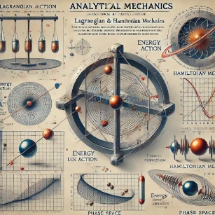
Analytical Mechanics: depicting Lagrangian and Hamiltonian mechanics with their respective principles
Core Architectural Frameworks
The Lagrangian approach shifts focus from vector force balance equations to scalar energy relations by evaluating a system’s configuration through an arbitrary set of generalized coordinates and generalized velocities. By defining the scalar Lagrangian function as the difference between the total kinetic energy and the potential energy:
$$L(q_i, \dot{q}_i, t) = T – V$$
Hamilton’s Principle of Least Action dictates that the true kinematical path traversed by a dynamic system between fixed temporal boundaries is a stationary point (extremum) of the action functional:
Applying the fundamental lemma of the calculus of variations translates this path extremization into the formal Euler-Lagrange equations of motion for each separate degree of freedom:
This layout eliminates holonomic constraint forces entirely from the configuration equations, avoiding complex geometric vector decompositions.
System Dynamics Derivation: Simple Pendulum
Below is the complete step-by-step structural derivation for a simple pendulum system using a single generalized coordinate, the angular displacement, evaluated at default system mass and length variables.
1. System Kinetic Energy:
$$T = \frac{1}{2} m l^2 \dot{\theta}^2 = 2.000 \dot{\theta}^2$$
2. System Potential Energy:
$$V = m g l (1 – \cos\theta) = 19.620 (1 – \cos\theta)$$
3. Formulated Lagrangian:
$$L = T – V = 2.000 \dot{\theta}^2 – 19.620 (1 – \cos\theta)$$
The Hamiltonian framework upgrades the tracking configuration from n second-order coordinate constraints to a symmetrical matrix of 2n first-order differential profiles. This transformation is initiated by taking the Legendre transform of the system Lagrangian, substituting the coordinate velocities with canonical conjugate momenta, explicitly defined as:
$$p_i = \frac{\partial L}{\partial \dot{q}_i}$$
The total scalar system energy profile is cast as the Hamiltonian function H:
$$H(q_i, p_i, t) = \sum_i p_i \dot{q}_i – L$$
Taking the differential variation of H directly yields Hamilton’s Canonical Equations of Motion:
This geometric restructuring tracks the system evolution through a continuous mathematical construct known as phase space, where the exact state of an isolated network maps onto a single coordinates tracking path over time.
Table of Contents
Key Concepts in Analytical Mechanics
Generalized Coordinates and Constraints
In complex mechanical systems, it is often inefficient to describe motion using standard Cartesian coordinates (x, y, z). Instead, generalized coordinates are used, which simplify the system by eliminating redundant variables and incorporating spatial limitations automatically.
Generalized Coordinates (qi): Any independent parameters that uniquely define the configuration of a system (e.g., angles, distances).
Degrees of Freedom (DOF): The number of independent variables required to specify the complete physical configuration of a system.
Constraints: Geometric or kinematic relationships between coordinates that reduce the total number of independent variables.
Holonomic Constraints: Relationships that can be expressed strictly as algebraic equations relating coordinates and time:
$$f(q_i, t) = 0$$
Non-Holonomic Constraints: Constraints that cannot be integrated into equations of coordinates alone, often expressed as non-integrable differentials or inequalities (e.g., rolling without slipping).
Lagrangian Mechanics
Definition: Lagrangian mechanics reformulates Newtonian mechanics by focusing on scalar energy values rather than vector force balancing. It is fundamentally based on Hamilton’s Principle of Least Action, which states that the path taken by a system between two configurations is the one for which the action integral is stationary.
Lagrangian Function (L):
$$L = T – V$$
Where:
T = Total kinetic energy of the system
V = Total potential energy of the system
Euler-Lagrange Equation: The dynamic equations of motion are derived by applying the variational calculus step to the Lagrangian functional for each coordinate qi:
Where the dot derivative over qi represents the generalized velocity (the explicit time derivative of the generalized coordinate).
Advantages: It simplifies the mathematical analysis for multi-body configurations containing complex constraint forces, and provides a seamless conceptual transition to quantum mechanics through Feynman’s path integral formulation.
Hamiltonian Mechanics
Definition: Hamiltonian mechanics is an alternative formulation focused on energy parameters that shifts the system mapping into a symmetrical phase space consisting of coordinates and conjugate momenta. It forms the foundation for statistical mechanics, quantum dynamics, and advanced orbital pathing.
Hamiltonian Function (H):
$$H = \sum_i p_i \dot{q}_i – L$$
Where pi represents the generalized conjugate momentum derived from the partial velocity derivative of the Lagrangian. For most conservative, time-independent systems, the Hamiltonian maps directly to the total mechanical energy:
These paired first-order differential equations replace Newton’s second-order vector equations, structuring a highly efficient layout for tracking state variables.
Principle of Least Action
The Principle of Least Action dictates that the actual path traversed by a dynamic system between times t1 and t2 is an extremum of the scalar action functional S:
This scalar optimization underpins the entirety of classical mechanics and serves as a primary link connecting macroscopic physics to modern field theories.
Sub-Areas of Study in Analytical Mechanics
Focus: Finding the specific functions and paths that minimize or maximize a given scalar functional over specified boundary constraints.
Key Topics:
The fundamental lemma of the calculus of variations.
Derivation and properties of the Euler-Lagrange differential equations.
Functional optimization containing integral constraints via Lagrange multipliers.
Applications: Brachistochrone problem stabilization, geodesic mapping on curved manifolds, and trajectory optimization in aerospace navigation.
Focus: Restructuring mechanical problems into arbitrary generalized coordinates to completely eliminate holonomic constraint forces from equations of motion.
Key Topics:
Formulation of the scalar Lagrangian function: L = T – V.
Identification and exploitation of cyclic (ignorable) coordinates.
D’Alembert’s principle and the formal definition of virtual work.
Focus: Mapping physical states into a continuous 2n-dimensional phase space using coordinate positions and canonical momentum variables simultaneously.
Key Topics:
The Legendre transform mapping formula: H = ∑ pi q̇i – L.
Derivation of Hamilton’s symmetric, first-order canonical equations of motion.
Liouville’s theorem proving the conservation of phase-space density volume over time.
Focus: Applying mathematical coordinate modifications in phase space that preserve the form of Hamilton’s equations while simplifying the underlying invariants.
Key Topics:
Symplectic matrix transformations and algebraic properties of Poisson Brackets.
The Hamilton-Jacobi equation mapping the path to a constant equilibrium configuration.
Action-angle variables for completely integrable periodic networks.
Applications: Advanced celestial perturbation calculations, chaotic transition boundary tracking, and forming the operators for quantum mechanics.
Symmetry and Gauge Invariance: Noether’s Theorem
The pinnacle achievement of the analytical mechanics framework is the mathematical unification of geometric symmetries with physical conservation laws, formalised via Noether’s Theorem.
If a system Lagrangian remains completely invariant under a continuous coordinate translation scaled by an infinitesimal parameter, the action integral exhibits a continuous symmetry mapping:
$$q_i \quad \rightarrow \quad q_i + \delta q_i$$
$$\delta L = \sum_i \left( \frac{\partial L}{\partial q_i} \delta q_i + \frac{\partial L}{\partial \dot{q}_i} \delta \dot{q}_i \right) = 0$$
Substituting the Euler-Lagrange differential relations into the variation equation yields:
$$\delta L = \sum_i \left[ \frac{d}{dt}\left(\frac{\partial L}{\partial \dot{q}_i}\right) \delta q_i + \frac{\partial L}{\partial \dot{q}_i} \frac{d}{dt}(\delta q_i) \right] = 0$$
$$\frac{d}{dt} \left[ \sum_i \frac{\partial L}{\partial \dot{q}_i} \delta q_i \right] = 0$$
This derivative proves that the scalar product enclosed in the brackets is an absolute invariant over time. Consequently:
Homogeneity of Time: If the Lagrangian is invariant under a continuous shift in the time coordinate, total system energy (H) is conserved:
$$\frac{\partial L}{\partial t} = 0$$
Homogeneity of Space: If the Lagrangian is invariant under spatial translations, total linear momentum (p) is conserved:
$$\frac{\partial L}{\partial x} = 0$$
Isotropy of Space: If the Lagrangian is invariant under spatial rotations, angular momentum matches a conserved constant value:
$$\frac{\partial L}{\partial \theta} = 0$$
Applications of Analytical Mechanics
Orbital Mechanics: Charting planetary paths and satellite configurations using energy optimization profiles.
Quantum Mechanics: Constructing the canonical foundation for quantum operators and Schrödinger’s wave mechanics.
Control Systems: Designing multi-jointed robotic linkages and spacecraft altitude trajectories subject to hard physical coordinates constraints.
General Relativity: Formulating the Einstein field equations via the variational principle applied to the Hilbert action.
Optimization Problems: Resolving high-dimensional mechanical layouts and material efficiency tracks using variational principles.
Five Examples on Analytical Mechanics
Example 1: Simple Harmonic Oscillator (Lagrangian Mechanics)
Problem: A system consists of a mass attached to a spring with a defined spring constant oscillating on a frictionless horizontal plane. Derive the dynamic equation of motion using the Lagrangian framework.
Solution:The scalar kinetic energy of the system is defined by:
$$T = \frac{1}{2} m \dot{x}^2$$The conservative potential energy stored in the spring is defined by:
$$V = \frac{1}{2} k x^2$$The system Lagrangian is constructed as the difference between kinetic and potential states:
$$L = T – V = \frac{1}{2} m \dot{x}^2 – \frac{1}{2} k x^2$$
Applying the foundational Euler-Lagrange equation for the coordinate variable:
$$\frac{d}{dt} \left( \frac{\partial L}{\partial \dot{x}} \right) – \frac{\partial L}{\partial x} = 0$$Evaluating the respective partial derivatives:
$$\frac{\partial L}{\partial \dot{x}} = m\dot{x} \quad \rightarrow \quad \frac{d}{dt}\left( m\dot{x} \right) = m\ddot{x}$$
$$\frac{\partial L}{\partial x} = -kx$$Substituting these derivatives back into the variational layout yields:
$$m\ddot{x} – (-kx) = 0$$
$$m\ddot{x} + kx = 0$$
Answer: The derived differential equation of motion tracks standard simple harmonic behavior:
$$m\ddot{x} + kx = 0$$
Example 2: Pendulum (Lagrangian Mechanics)
Problem: Derive the second-order differential equation of motion for a simple pendulum of defined length and mass using its angular configuration parameter.
Solution:The translational kinetic energy mapped along the arc trajectory matches:
$$T = \frac{1}{2} m l^2 \dot{\theta}^2$$The gravitational potential energy relative to the equilibrium datum matches:
$$V = mgl(1 – \cos\theta)$$The calculated system Lagrangian is:
$$L = \frac{1}{2} m l^2 \dot{\theta}^2 – mgl(1 – \cos\theta)$$
Applying the Euler-Lagrange framework along the generalized coordinate variable:
$$\frac{d}{dt} \left( \frac{\partial L}{\partial \dot{\theta}} \right) – \frac{\partial L}{\partial \theta} = 0$$Evaluating the respective partial derivatives:
$$\frac{\partial L}{\partial \dot{\theta}} = ml^2\dot{\theta} \quad \rightarrow \quad \frac{d}{dt}\left( ml^2\dot{\theta} \right) = ml^2\ddot{\theta}$$
$$\frac{\partial L}{\partial \theta} = -mgl\sin\theta$$Substituting these derivatives back into the variational layout yields:
$$ml^2\ddot{\theta} – (-mgl\sin\theta) = 0$$
$$ml^2\ddot{\theta} + mgl\sin\theta = 0$$
Answer: Factoring out common scaling variables simplifies the expression to the final ordinary differential equation:
$$\ddot{\theta} + \frac{g}{l}\sin\theta = 0$$
Example 3: Hamiltonian for Free Particle
Problem: Find the canonical Hamiltonian expression for an unconstrained free particle moving in a one-dimensional reference frame.
Solution:Since no external fields exist, potential energy equals zero, yielding the Lagrangian:
$$L = \frac{1}{2} m \dot{x}^2$$The canonical conjugate momentum variable is explicitly defined as:
$$p = \frac{\partial L}{\partial \dot{x}} = m\dot{x}$$Inverting this relation translates the velocity variable into momentum phase coordinates:
$$\dot{x} = \frac{p}{m}$$
Applying the Legendre transform to shift system variables from coordinate velocities to canonical phase spaces:
$$H = p\dot{x} – L$$
$$H = p\left(\frac{p}{m}\right) – \frac{1}{2}m\left(\frac{p}{m}\right)^2$$
$$H = \frac{p^2}{m} – \frac{p^2}{2m}$$
Answer: The configured Hamiltonian represents the total mechanical energy state:
$$H = \frac{p^2}{2m}$$
Example 4: Particle in Gravitational Field
Problem: A particle shifts coordinates vertically inside a uniform gravitational field. Determine the final system Hamiltonian expression.
Solution:Setting height as the generalized displacement coordinate defines the system Lagrangian:
$$L = \frac{1}{2} m \dot{h}^2 – mgh$$Calculating the corresponding linear momentum variable:
$$p = \frac{\partial L}{\partial \dot{h}} = m\dot{h} \quad \rightarrow \quad \dot{h} = \frac{p}{m}$$
Transforming the functions via the Legendre expression:
$$H = p\dot{h} – L$$
$$H = p\left(\frac{p}{m}\right) – \left[\frac{1}{2}m\left(\frac{p}{m}\right)^2 – mgh\right]$$
$$H = \frac{p^2}{m} – \frac{p^2}{2m} + mgh$$
Answer: The isolated Hamiltonian function returns the sum of kinetic and potential coordinates:
$$H = \frac{p^2}{2m} + mgh$$
Example 5: Charged Particle in Magnetic Field
Problem: Formulate the Hamiltonian of an isolated particle interacting with an unconstrained electromagnetic vector potential field.
Solution:The structural coupling introduces velocity-dependent variations. The true canonical conjugate momentum resolves to:
$$\mathbf{p} = m\mathbf{v} + q\mathbf{A}$$Isolating the mechanical velocity vector yields the mapping expression:
$$\mathbf{v} = \frac{1}{m}(\mathbf{p} – q\mathbf{A})$$Applying the Legendre transformation matrix systematically removes velocity vectors, replacing them with canonical momentum phase coordinates:
$$H = \frac{1}{2m}(\mathbf{p} – q\mathbf{A})^2$$
Answer: The structured Hamiltonian maps to:
$$H = \frac{1}{2m}(\mathbf{p} – q\mathbf{A})^2$$
Why Study Analytical Mechanics
Advanced Framework for Motion
Analytical mechanics reformulates classical mechanics using principles of energy and generalized coordinates. Students study Lagrangian and Hamiltonian methods to describe motion elegantly. These approaches simplify complex systems and constraints. They offer deeper insight into physical laws and symmetries.
Mathematical Rigor and Elegance
Students use calculus of variations and differential geometry to explore physical systems. This develops a more abstract and unified understanding of mechanics. Analytical mechanics promotes mathematical creativity and precision. It prepares students for advanced physics and applied mathematics.
Applications to Modern Physics
Analytical mechanics is foundational for quantum mechanics, statistical mechanics, and field theory. Students learn how Hamiltonian dynamics links to quantum systems. This knowledge supports theoretical research and graduate study. It connects classical foundations to cutting-edge science.
Conservation Laws and Symmetry
Students explore how symmetries lead to conservation of energy, momentum, and angular momentum. Noether’s theorem provides a powerful framework for understanding physical invariants. These insights unify different areas of physics. They enhance theoretical and conceptual clarity.
Modeling Complex Systems
Analytical mechanics is used to model planetary motion, pendulums, and mechanical systems with constraints. Students apply it to robotics, spacecraft, and molecular dynamics. This supports interdisciplinary problem-solving. It fosters innovation in science and engineering applications.
Conclusion on Analytical Mechanics
Analytical Mechanics offers exceptionally powerful tools for solving complex physical problems using unified energy principles. By shifting configuration metrics away from coordinate force vectors to localized scalar frameworks, the Lagrangian and Hamiltonian formulations simplify calculations across multidimensional systems, providing an indispensable foundation for theoretical physics and mathematical engineering tracks.
Analytical Mechanics — FAQ
What is analytical mechanics, and how does it differ from Newtonian mechanics?
Analytical mechanics is a more general and elegant reformulation of classical mechanics that uses powerful mathematical tools such as generalized coordinates, Lagrangians, and Hamiltonians. While Newtonian mechanics focuses on forces and vector equations like $\vec{F} = m\vec{a}$, analytical mechanics works with scalar quantities such as kinetic and potential energy and uses variational principles to derive equations of motion. Both describe the same physics but with different, often more flexible, formalisms.
What are generalized coordinates, and why are they useful in analytical mechanics?
Generalized coordinates are a set of variables chosen to describe the configuration of a system in the most convenient way, which may or may not be ordinary Cartesian coordinates. For example, angles, distances along a track, or any other independent parameters can be used. By adopting generalized coordinates, analytical mechanics allows you to describe complex systems with constraints more naturally and to reduce the number of equations you need to solve.
What is the Lagrangian, and how does the Euler–Lagrange equation describe motion?
The Lagrangian is defined as $L = T - V$, the difference between a system’s kinetic energy $T$ and potential energy $V$ expressed in terms of generalized coordinates and velocities. The Euler–Lagrange equation is a differential equation obtained by requiring that the action (the time integral of $L$) be stationary. Solving the Euler–Lagrange equations gives the equations of motion without having to explicitly resolve all forces, making it very powerful for systems with constraints and symmetries.
What is meant by the principle of least action in analytical mechanics?
The principle of least action states that the actual path taken by a system between two configurations is the one for which the action, defined as the integral of the Lagrangian over time, is stationary (usually a minimum compared with nearby paths). This variational principle provides a unifying way to derive the equations of motion and highlights deep connections between mechanics, optics, and even quantum physics.
What is Hamiltonian mechanics, and how is it related to the Lagrangian formulation?
Hamiltonian mechanics is another reformulation of classical mechanics in which the state of a system is described by generalized coordinates and conjugate momenta instead of coordinates and velocities. The Hamiltonian, often equal to the total energy, generates the time evolution through Hamilton’s equations. It can be derived from the Lagrangian and is especially useful in advanced topics such as canonical transformations, statistical mechanics, and quantum mechanics.
How does analytical mechanics handle constraints more easily than Newtonian mechanics?
In Newtonian mechanics, constraints often appear as additional force components that must be determined explicitly. Analytical mechanics incorporates constraints directly into the choice of generalized coordinates and into the Lagrangian. This approach can eliminate constraint forces from the equations of motion or treat them systematically using methods such as Lagrange multipliers, greatly simplifying the analysis of complex systems like pendulums, linkages, and rolling bodies.
What role do symmetries and conservation laws play in analytical mechanics?
Analytical mechanics makes the connection between symmetries and conservation laws very explicit. When the Lagrangian does not change under a particular transformation, such as a shift in time, space, or angle, a corresponding quantity is conserved (energy, linear momentum, or angular momentum). This idea is formalized by Noether’s theorem and is central to modern theoretical physics, from classical fields to particle physics and general relativity.
Why is analytical mechanics important for university-level physics and engineering studies?
Analytical mechanics provides a systematic framework that scales well from simple textbook problems to complex, realistic systems. It sharpens your skills in mathematical modeling, differential equations, and vector and tensor calculus, all of which are essential in advanced mechanics, electromagnetism, quantum physics, and many engineering disciplines. Learning analytical mechanics early gives you a language that is widely used across modern theoretical and applied physics.
What mathematical background helps in learning analytical mechanics?
A solid foundation in calculus (including partial derivatives), differential equations, vector calculus, and linear algebra is very helpful for analytical mechanics. Familiarity with coordinate transformations, gradients, and basic variational ideas will also make the concepts less intimidating. The Prep4Uni materials highlight how each piece of mathematics connects to physical reasoning so that both grow together.
How does analytical mechanics connect to quantum mechanics and modern physics?
Many of the core ideas in quantum mechanics and modern field theories are natural extensions of analytical mechanics. The Hamiltonian becomes the central operator that governs quantum time evolution, and path integral formulations build directly on the principle of action. Studying analytical mechanics at pre-university level makes the transition to quantum mechanics and advanced courses smoother because you already speak the language of Lagrangians, Hamiltonians, and symmetries.
Is analytical mechanics only for very advanced students, or can pre-university students benefit from it?
Pre-university students can definitely benefit from an intuitive introduction to analytical mechanics. Even without full mathematical detail, learning how generalized coordinates, Lagrangians, and conservation laws fit together deepens your understanding of familiar topics like energy and momentum. It also gives you a preview of the methods used in university physics, making the first-year mechanics and mathematical physics courses feel more familiar and less abstract.
How can the analytical mechanics section on Prep4Uni help me prepare for future studies?
The Prep4Uni analytical mechanics section aims to bridge the gap between school-level Newtonian mechanics and university-level theoretical physics. It introduces key concepts through diagrams, energy-based reasoning, and step-by-step derivations, then connects them to related topics such as calculus, linear algebra, and numerical methods. By engaging with these materials, you build both conceptual insight and mathematical readiness for future physics or engineering degrees.
Mechanics Through the Lens of Energy, Variational Principles, and Abstraction
Analytical Mechanics: Review Questions and Answers
Answer: Analytical mechanics reformulates classical mechanics using energy functions and variational principles rather than force vectors. Unlike Newtonian mechanics, which relies on $\vec{F}=m\vec{a}$ and vector forces, it employs generalized coordinates and functions such as the Lagrangian and Hamiltonian, allowing for more elegant and flexible problem-solving, especially in complex or constrained systems.
Answer: The Lagrangian is defined as the difference between a system’s kinetic and potential energies ($L = T – V$). It serves as the core function in the Lagrangian formulation, where applying the principle of least action leads to the Euler-Lagrange equations, which govern the dynamics of the system.
Answer: The Euler-Lagrange equations are derived by applying the principle of least action, which states that the actual path taken by a system minimizes the action integral. These equations provide the necessary conditions for this minimization and yield the equations of motion for the system in terms of its generalized coordinates.
Answer: The principle of least action asserts that the path a system takes between two states is the one for which the action integral (the time integral of the Lagrangian) is minimized. This principle unifies various laws of physics into a single variational framework, offering deep insights into the conservation laws and symmetries inherent in physical systems.
Answer: The Hamiltonian is a function that typically represents the total energy of the system, defined through a Legendre transformation of the Lagrangian. It provides an alternative formulation of mechanics—Hamiltonian mechanics—where the evolution of a system is described by Hamilton’s equations, offering a powerful framework especially useful in statistical mechanics and quantum theory.
Answer: Hamilton’s equations are a set of first-order differential equations derived from the Hamiltonian. They describe the time evolution of generalized coordinates and conjugate momenta, providing a symmetrical and often more tractable formulation of the dynamics, particularly in systems with complex interactions or conserved quantities.
Answer: The Legendre transformation is a mathematical procedure that converts a function of one set of variables into a function of another set by replacing velocities with conjugate momenta. This transformation is key in transitioning from the Lagrangian (energy difference) to the Hamiltonian (total energy) formulation, linking the two approaches in analytical mechanics.
Answer: Analytical mechanics offers several advantages, including the ability to handle systems with constraints more naturally through generalized coordinates, a unified approach via variational principles, and more straightforward connections to conservation laws and symmetries. These benefits make it particularly useful for complex and multi-body systems.
Answer: According to Noether’s theorem, every continuous symmetry of the action corresponds to a conservation law. In analytical mechanics, symmetries in the Lagrangian or Hamiltonian imply the conservation of quantities like energy, momentum, or angular momentum, providing deep insights into the invariant properties of physical systems.
Answer: Generalized coordinates allow the description of a system’s configuration in terms of the minimum number of independent variables, which can be tailored to the system’s constraints. This flexibility simplifies the mathematical formulation and solution of complex mechanical problems, making analytical mechanics a powerful tool for theoretical and applied physics.
Analytical Mechanics: Thought-Provoking Questions and Answers
Answer: Analytical mechanics, through its emphasis on variational principles and energy functions, serves as a bridge to modern theoretical frameworks such as quantum mechanics and field theory. Its methodologies underpin the development of path integrals and gauge theories, offering a unifying language that transcends classical dynamics and aids in the exploration of fundamental interactions in nature.
Answer: The principle of least action is central to the path integral formulation, where every possible path contributes to the quantum amplitude, weighted by an exponential of the classical action. This connection reveals that classical paths dominate in the macroscopic limit, while quantum effects arise from the interference of multiple trajectories, unifying classical and quantum descriptions.
Answer: Generalized coordinates simplify the description of systems with constraints, allowing for more efficient modeling of multi-body dynamics, articulated mechanisms, and robotic motion. By reducing the number of independent variables, engineers can develop more accurate simulations, optimize control algorithms, and design systems that operate with greater precision in complex environments.
Answer: Traditional analytical mechanics is best suited for conservative systems where energy is conserved. In dissipative systems, friction and non-conservative forces complicate the formulation. These challenges can be addressed by extending the formalism to include non-conservative potentials or using generalized methods such as Rayleigh’s dissipation function, though these adaptations often require more sophisticated mathematical tools.
Answer: Symmetries in a system, as formalized by Noether’s theorem, imply that invariant properties result in conserved quantities. This deep connection suggests that the laws of physics are governed by underlying symmetries, which not only simplify the mathematical formulation of physical theories but also hint at the fundamental structure and order of the universe.
Answer: Alternative variational principles that incorporate non-conservative forces or account for dissipative processes may reveal new aspects of system dynamics. These modified principles could help describe phenomena such as turbulence, self-organization, or phase transitions in complex systems, potentially leading to breakthroughs in understanding emergent behaviors in nature.
Answer: Enhanced computational power and sophisticated numerical algorithms allow for the efficient simulation of high-dimensional and nonlinear systems, where analytical solutions are intractable. These advances enable researchers to explore complex dynamics, optimize action integrals, and predict system behavior with high accuracy, thereby broadening the scope and applicability of analytical mechanics.
Answer: The Hamiltonian framework provides a natural description of system dynamics in terms of energy and momentum, which can be integrated with control theory to design optimal control strategies. By exploiting the symplectic structure and conservation laws, engineers can develop robust algorithms for real-time system stabilization, energy management, and trajectory optimization in fields such as robotics and aerospace.
Answer: Analytical mechanics lays the groundwork for quantum theory through its variational principles and action-based formulations. Concepts such as the Hamiltonian and Lagrangian are directly carried over into quantum mechanics, facilitating the transition from classical determinism to quantum probabilism. This bridge helps elucidate how classical behavior emerges from quantum rules and guides the development of quantum field theories.
Answer: Symplectic geometry provides a rigorous mathematical framework for understanding the structure of phase space in Hamiltonian mechanics. By leveraging these geometric insights, researchers can uncover invariants, study stability and chaos, and develop new methods for integrating equations of motion, thereby deepening our comprehension of dynamical systems and enhancing analytical techniques.
Answer: Analyzing chaotic systems through the lens of analytical mechanics allows for the identification of underlying order in seemingly random behavior. By comparing theoretical predictions with experimental data, scientists can refine models, understand the sensitivity to initial conditions, and develop statistical descriptions that capture the essence of chaos, ultimately contributing to advances in fields such as meteorology and plasma physics.
Answer: Educational strategies can be enhanced by integrating computational tools, interactive simulations, and problem-based learning into the curriculum. Emphasizing the connections between analytical mechanics, modern physics, and real-world applications helps students grasp abstract concepts, develop critical problem-solving skills, and gain a deeper appreciation for the unifying principles that underpin diverse physical phenomena.
Analytical Mechanics: Advanced Numerical Practice Suite
Problem 1: Two-Body Atwood Machine via Generalized Coordinates
Scenario: A frictionless pulley suspends two masses hanging vertically in a uniform gravitational field. The string is inextensible and has a fixed total length. Derive the exact acceleration of the system using a single generalized coordinate.
Quantitative Setup: Let the positions of the two masses relative to the pulley axis be tracked by spatial coordinates:
$$x_1 \quad \text{and} \quad x_2$$
The holonomic string length constraint satisfies the linear relation:
$$x_1 + x_2 = l \quad \rightarrow \quad \dot{x}_1 = -\dot{x}_2$$
We choose the position of the first mass as our sole generalized coordinate:
$$q = x_1 \quad \rightarrow \quad \dot{q} = \dot{x}_1$$
Mathematical Formulation: The total kinetic energy of the system is the sum of both moving masses:
$$T = \frac{1}{2} m_1 \dot{x}_1^2 + \frac{1}{2} m_2 \dot{x}_2^2 = \frac{1}{2}(m_1 + m_2)\dot{q}^2$$
The potential energy relative to the pulley datum is:
$$V = -m_1 g x_1 – m_2 g x_2 = -m_1 g q – m_2 g (l – q)$$
The configured Lagrangian function is:
$$L = T – V = \frac{1}{2}(m_1 + m_2)\dot{q}^2 + m_1 g q + m_2 g (l – q)$$
Variational Execution: Computing the partial derivatives required for the Euler-Lagrange expression:
$$\frac{\partial L}{\partial \dot{q}} = (m_1 + m_2)\dot{q} \quad \rightarrow \quad \frac{d}{dt}\left( \frac{\partial L}{\partial \dot{q}} \right) = (m_1 + m_2)\ddot{q}$$
$$\frac{\partial L}{\partial q} = m_1 g – m_2 g = (m_1 – m_2)g$$
Assembling the final equation of motion:
$$(m_1 + m_2)\ddot{q} – (m_1 – m_2)g = 0$$
Answer & Verification: Solved explicitly for system acceleration:
$$\ddot{q} = \left( \frac{m_1 – m_2}{m_1 + m_2} \right) g$$
Problem 2: Central Potential Orbit Canonical Momenta
Scenario: A particle of mass moves in a plane under the influence of a spherically symmetric, conservative central potential function. Formulate the Lagrangian in polar coordinates and solve for the conserved momentum constant.
Quantitative Setup: The position is mapped using generalized radius and angular variables:
$$q_1 = r \quad \text{and} \quad q_2 = \theta$$
The velocity squared in planar polar coordinates expands to:
$$v^2 = \dot{r}^2 + r^2 \dot{\theta}^2$$
Mathematical Formulation: The kinetic energy and Lagrangian functions are expressed as:
$$T = \frac{1}{2} m (\dot{r}^2 + r^2 \dot{\theta}^2)$$
$$L = \frac{1}{2} m (\dot{r}^2 + r^2 \dot{\theta}^2) – V(r)$$
Variational Execution: Evaluating the angular equation of motion via Euler-Lagrange equations:
$$\frac{\partial L}{\partial \dot{\theta}} = m r^2 \dot{\theta} \quad \rightarrow \quad \frac{d}{dt}(m r^2 \dot{\theta})$$
$$\frac{\partial L}{\partial \theta} = 0$$
Because the angular coordinate is cyclic (absent from the Lagrangian function), its corresponding canonical conjugate momentum is an absolute constant of motion:
$$p_{\theta} = \frac{\partial L}{\partial \dot{\theta}} = m r^2 \dot{\theta} = \text{const}$$
Answer & Verification: The angular momentum parameter remains completely invariant over the entire trajectory timeline:
$$\frac{d}{dt}(p_{\theta}) = 0 \quad \rightarrow \quad L_z = m r^2 \dot{\theta} = \text{const}$$