
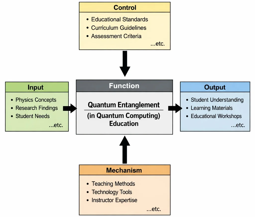
Quantum entanglement education, within a modern quantum computing framework, operates as a rigorous systems-engineering discipline that translates abstract quantum mechanical nonlocality into practical computational and cryptographic architectures. In this IDEF0 functional model, learners begin with foundational inputs: state vector formalisms, tensor product spaces, the postulates of quantum measurement, and common student misconceptions regarding faster-than-light signaling. Governed by formal controls—the non-signaling theorem, Bell inequality bounds, and fault-tolerant error budgets—students explore how non-classical correlations are generated, verified, and manipulated. Supported by experimental mechanisms including photonic down-conversion testbeds, superconducting transmon circuits, and interactive numerical simulators, students develop the capacity to design entanglement-driven algorithms, implement quantum key distribution (QKD) protocols, and evaluate distributed quantum networks.
Quantum entanglement represents a fundamental resource in quantum information science, establishing non-local state correlations between qubits that have no counterpart in classical probability theory. Whereas an \(n\)-bit classical register exists in one deterministic configuration at any given instant, an \(n\)-qubit entangled register spans a \(2^n\)-dimensional complex Hilbert space. By synthesizing principles across quantum gates and circuits, multi-qubit transformations such as the controlled-NOT (CNOT) gate convert product states into maximally entangled Bell states, creating the core operational framework for Shor's algorithm, Grover's search, and distributed quantum teleportation.
Mastering entanglement requires strong mathematical grounding in abstract linear algebra from pure mathematics and stochastic modeling from probability and statistics. Entanglement operates in close synergy with quantum superposition and single-qubit state control via physical qubits. In quantum communications, entanglement provides physics-based cryptographic guarantees: any eavesdropping attempt inevitably alters the shared quantum state, inducing measurable perturbations in Bell-state correlation metrics.
Beyond quantum computation, entanglement interfaces directly with broader STEM disciplines and emerging technologies. In artificial intelligence and machine learning, parameterized quantum circuits utilizing entangled feature spaces accelerate high-dimensional classification and tensor network contractions. Furthermore, in autonomous systems and robotics, entangled photon sensors provide Heisenberg-limited precision for sub-diffraction optical metrology, inertial navigation, and deep-space telemetry across space exploration networks.
Need the foundational physical mechanics? Explore the physics-level module on Quantum Entanglement in Modern Quantum Mechanics.
Mathematical Formalism of Composite Entangled States
In quantum mechanics, a bipartite quantum system comprising subsystem \(A\) and subsystem \(B\) is defined over the tensor product of their respective Hilbert spaces, \(\mathcal{H}_{AB} = \mathcal{H}_A \otimes \mathcal{H}_B\). A state \(|\psi_{AB}\rangle\) is strictly defined as separable if and only if it can be factored into an isolated tensor product of individual subsystem states:
$$|\psi_{\text{sep}}\rangle = |\phi_A\rangle \otimes |\chi_B\rangle$$Conversely, a quantum state is entangled if it cannot be written as a product state. For a two-qubit system spanned by the computational basis \(\{|00\rangle, |01\rangle, |10\rangle, |11\rangle\}\), a general pure entangled state is expressed as:
General Two-Qubit State Vector:
$$|\psi_{AB}\rangle = c_{00}|00\rangle + c_{01}|01\rangle + c_{10}|10\rangle + c_{11}|11\rangle \quad \text{where } c_{ij} \in \mathbb{C}$$Subject to the Born normalization condition: \(|c_{00}|^2 + |c_{01}|^2 + |c_{10}|^2 + |c_{11}|^2 = 1\).
The canonical maximally entangled two-qubit states form the complete orthonormal Bell Basis (also known as EPR pairs):
The Four Orthonormal Bell States:
$$|\Phi^+\rangle = \frac{1}{\sqrt{2}}(|00\rangle + |11\rangle) \qquad |\Phi^-\rangle = \frac{1}{\sqrt{2}}(|00\rangle - |11\rangle)$$ $$|\Psi^+\rangle = \frac{1}{\sqrt{2}}(|01\rangle + |10\rangle) \qquad |\Psi^-\rangle = \frac{1}{\sqrt{2}}(|01\rangle - |10\rangle)$$In \(|\Phi^+\rangle\), measurement of qubit \(A\) in the \(\{|0\rangle, |1\rangle\}\) basis yielding \(|0\rangle\) instantly forces qubit \(B\) to collapse into \(|0\rangle\) with certainty (\(P=1.0\)), regardless of spatial separation.
Fundamental Epistemological & Physical Properties
1. Nonlocality & The Non-Signaling Theorem
Entangled particles exhibit instantaneous non-local spatial correlations upon measurement. However, because local measurement outcomes are intrinsically random (governed by the Born rule), no controllable binary signal or message can be transmitted across space faster than the speed of light. To decode or reconstruct information (as in quantum teleportation), observers must transmit classical measurement outcomes over conventional channels, adhering strictly to special relativity.
2. Bell's Theorem & CHSH Inequality Violations
In 1964, John Stewart Bell proved that no physical theory based on local hidden variables can reproduce the statistical predictions of quantum mechanics. The Clauser-Horne-Shimony-Holt (CHSH) inequality establishes that for any classical local realistic theory, the correlation parameter \(S\) is strictly bounded: $$|S_{\text{classical}}| \le 2$$ Quantum mechanics predicts, and experiments consistently confirm, a maximum violation reaching the Tsirelson Bound: $$S_{\text{quantum}} = 2\sqrt{2} \approx 2.828$$ ruling out local deterministic hidden variables.
3. The No-Cloning Theorem
Formally proved by Wootters, Zurek, and Dieks in 1982, the No-Cloning Theorem states that unitary quantum mechanics prohibits the creation of an identical copy of an arbitrary unknown quantum state: $$U(|\psi\rangle \otimes |0\rangle) \ne |\psi\rangle \otimes |\psi\rangle$$ This linear algebraic constraint ensures the fundamental security of quantum cryptography: an eavesdropper cannot tap a quantum communication channel by cloning carrier photons without introducing detectable perturbation.
Visualizing Quantum Entanglement: The Marriage Analogy
To build conceptual intuition before analyzing complex tensor formulations, examine how non-separable correlations, state collapse, and environmental decoherence operate in this story-driven visual model:
Physical Realizations & Frontier Technological Applications
Entanglement is generated across diverse physical substrates, driving multiple modern quantum technologies:
| Physical Architecture | Generation & Control Mechanism | Primary Engineering Application |
|---|---|---|
| Photonic Down-Conversion | Spontaneous Parametric Down-Conversion (SPDC) in nonlinear crystals (BBO, KTP) splitting pump photons into polarization-entangled pairs. | Long-distance free-space quantum satellite downlinks and fiber QKD networks (Ekert E91 protocol). |
| Superconducting Transmons | Microwave resonator bus coupling Josephson junction circuits at \(15 \text{ mK}\) to execute two-qubit cross-resonance gates. | On-chip algorithm execution (VQE, QAOA) and surface-code logical qubit error correction. |
| Trapped Ion Arrays | Linear Paul traps suspending ions; coupled vibrational modes (phonons) driven by Raman laser pulses execute Mølmer-Sørensen gates. | High-fidelity multi-qubit entanglement registers with long coherence times (\(T_2 \gt 1 \text{ s}\)). |
| Quantum Repeaters | Atomic gas or solid-state rare-earth crystal memories storing photons, utilizing Bell-state measurements for entanglement swapping. | Overcoming exponential fiber optical attenuation to enable continental-scale quantum internets. |
Interactive Entanglement Transmission & Fiber Loss Simulator
Simulate paired photon transmission over silica optical fiber (0 to 100 km). Analyze how fiber attenuation (\(\text{dB/km}\)) and detector quantum efficiency dictate the surviving entangled coincidence rate:
Interactive Review Checkpoints
Click each question to toggle the detailed technical model answer and evaluate your conceptual grasp:
Review Checkpoint 1: Why does instantaneous state collapse strictly forbid superluminal signaling?
Review Checkpoint 2: How does the Ekert (E91) QKD protocol detect eavesdropping (Eve)?
Frequently Asked Questions on Quantum Entanglement
1. What is quantum entanglement in accessible terms?
Quantum entanglement is a physical phenomenon where two or more particles share a unified, interdependent quantum state such that the physical properties of one cannot be described independently of the other. Measuring one particle immediately dictates the state of its entangled partner, even if they are light-years apart, exhibiting correlations far stronger than any classical statistical process allows.
2. How does entanglement differ from ordinary classical correlations?
Classical correlations stem from shared past conditions carrying pre-determined, fixed states (such as cutting a pair of shoes and placing each into a separate sealed box: finding the left shoe immediately reveals the other box holds the right shoe). Entangled particles carry no pre-determined outcomes before measurement; their properties remain in a coherent quantum superposition until the measurement interaction forces a definite outcome.
3. Why are quantum repeaters required for long-distance terrestrial quantum networks?
Optical fibers exhibit intrinsic Rayleigh scattering and material absorption (typically \(\sim 0.2 \text{ dB/km}\) at \(1550 \text{ nm}\)), meaning photon transmission decays exponentially with distance. In classical telecom, optical amplifiers amplify signals by creating copies. In quantum networks, the No-Cloning Theorem forbids copying unknown photon states. Quantum repeaters solve this by establishing entanglement across short fiber segments and using entanglement swapping via Bell-state measurements to stitch distant nodes together without measuring the quantum key.
Comprehensive Entanglement Practice Modules
Part A: Core Foundational Review Questions
1. Why does the "two envelopes with coloured cards" analogy fail to capture true quantum entanglement?
2. For a spin-singlet state \(|\Psi^-\rangle = \frac{1}{\sqrt{2}}(|01\rangle - |10\rangle)\), what is measured on particle B if particle A is measured as spin-up along axis \(\hat{z}\)?
3. In quantum metrology, how does entanglement surpass the Standard Quantum Limit (SQL)?
Part B: Analytical & Scenario-Based Inquiry
1. How does quantum entanglement change our understanding of physical reality and locality?
2. What technical mechanisms allow quantum entanglement to enable modular quantum computing architectures?
Part C: Step-by-Step Quantitative Problems
Problem 1: Maximally Entangled State Measurement Projection
Scenario: Two qubits are prepared in the canonical Bell state \(|\Phi^+\rangle = \frac{1}{\sqrt{2}}(|00\rangle + |11\rangle)\). If qubit \(A\) is measured in the computational basis and found in state \(|0\rangle\), compute the conditional probability that qubit \(B\) will also be measured in state \(|0\rangle\).
Step-by-Step Derivation:
$$ \begin{aligned} |\Phi^+\rangle &= \frac{1}{\sqrt{2}}|00\rangle + \frac{1}{\sqrt{2}}|11\rangle \\ \text{Projector on Qubit } A: P_0 &= |0\rangle\langle 0| \otimes I \\ |\psi_{\text{post}}\rangle &= \frac{P_0|\Phi^+\rangle}{\sqrt{\langle\Phi^+|P_0|\Phi^+\rangle}} = \frac{\frac{1}{\sqrt{2}}|00\rangle}{\sqrt{1/2}} = |00\rangle = |0\rangle_A \otimes |0\rangle_B \\ P(0_B | 0_A) &= |\langle 0_B|0_B\rangle|^2 = 1.0 = 100\% \end{aligned} $$Answer & Conclusion: The measurement projects qubit \(B\) into \(|0\rangle\) with certainty (probability = \(1.0\) or \(100\%\)).
Problem 2: SPDC Photonic Pair Generation and Coincidence Detection
Scenario: A nonlinear spontaneous parametric down-conversion source generates \(R_{\text{gen}} = 10^6 \text{ photon pairs/s}\). Both photons pass through independent detectors with single-photon quantum efficiency \(\eta = 40.0\%\) (\(0.40\)). Calculate the rate of coincident pair detections per second.
Step-by-Step Derivation:
$$ \begin{aligned} \eta_{\text{pair}} &= \eta_A \times \eta_B = 0.40 \times 0.40 = 0.16 \quad (16.0\%) \\ R_{\text{detected}} &= R_{\text{gen}} \times \eta_{\text{pair}} = 10^6 \times 0.16 = 160{,}000 \text{ pairs/s} \end{aligned} $$Answer & Conclusion: The system records \(160{,}000 \text{ detected coincident pairs per second}\).
Problem 3: CHSH Inequality Bell-Violation Percentage
Scenario: An experimental Bell test records a CHSH correlation parameter of \(S_{\text{meas}} = 2.60\). Given that the local realistic classical limit is \(S_{\text{class}} = 2.00\), determine the percentage excess by which quantum nonlocality violates the classical bound.
Step-by-Step Derivation:
$$ \begin{aligned} \Delta S &= S_{\text{meas}} - S_{\text{class}} = 2.60 - 2.00 = 0.60 \\ \text{Percentage Excess} &= \left( \frac{\Delta S}{S_{\text{class}}} \right) \times 100\% = \left( \frac{0.60}{2.00} \right) \times 100\% = 30.0\% \end{aligned} $$Answer & Conclusion: The experimental result violates the classical threshold by \(30.0\%\).
Problem 4: Optical Fiber Attenuation and Entanglement Transmission
Scenario: Telecom fiber exhibits an attenuation coefficient of \(\alpha = 0.20 \text{ dB/km}\) at \(1550 \text{ nm}\). For a point-to-point fiber span of \(d = 60.0 \text{ km}\), calculate the total attenuation in decibels and the resulting transmission probability \(T = 10^{-L/10}\).
Step-by-Step Derivation:
$$ \begin{aligned} L &= \alpha \times d = 0.20 \text{ dB/km} \times 60.0 \text{ km} = 12.0 \text{ dB} \\ T &= 10^{-12.0 / 10} = 10^{-1.2} \approx 0.0630957 \approx 6.31\% \end{aligned} $$Answer & Conclusion: Fiber transmission efficiency is approximately \(6.31\%\) (attenuation: \(12.0 \text{ dB}\)).
Problem 5: Entanglement State Fidelity Shortfall
Scenario: A quantum network requires a minimum state fidelity of \(F_{\text{req}} = 95.0\%\) (\(0.95\)) relative to \(|\Phi^+\rangle\). State tomography reveals a measured fidelity of \(F_{\text{meas}} = 0.930\). Determine the relative shortfall percentage.
Step-by-Step Derivation:
$$ \begin{aligned} \Delta F &= F_{\text{req}} - F_{\text{meas}} = 0.950 - 0.930 = 0.020 \\ \text{Shortfall} &= \left( \frac{\Delta F}{F_{\text{req}}} \right) \times 100\% = \left( \frac{0.020}{0.950} \right) \times 100\% \approx 2.105\% \end{aligned} $$Answer & Conclusion: State fidelity shows a relative shortfall of approximately \(2.11\%\).
Problem 6: Cumulative Multi-Qubit Circuit Gate Fidelity
Scenario: An entangling circuit algorithm executes \(N = 100\) sequential two-qubit logic gates. Each gate operates with an error rate of \(\epsilon = 2.0\%\) (\(F_g = 0.98\)). Assuming independent Markovian errors, calculate the overall circuit success probability.
Step-by-Step Derivation:
$$ \begin{aligned} F_{\text{total}} &= (F_g)^N = (0.98)^{100} \\ \ln(F_{\text{total}}) &= 100 \times \ln(0.98) \approx 100 \times (-0.0202027) \approx -2.02027 \\ F_{\text{total}} &= e^{-2.02027} \approx 0.13262 \end{aligned} $$Answer & Conclusion: Overall circuit fidelity falls to \(13.26\%\) without quantum error correction.
Problem 7: Exponential Quantum Decoherence Lifetime Survival
Scenario: An entangled pair stored in an atomic quantum memory undergoes decoherence according to \(P(t) = e^{-t/\tau}\), where the characteristic coherence time is \(\tau = 150.0 \ \mu\text{s}\). Calculate the survival probability of the entangled state at \(t = 300.0 \ \mu\text{s}\).
Step-by-Step Derivation:
$$ \begin{aligned} \frac{t}{\tau} &= \frac{300.0 \ \mu\text{s}}{150.0 \ \mu\text{s}} = 2.0 \\ P(300) &= e^{-2.0} \approx 0.135335 \approx 13.53\% \end{aligned} $$Answer & Conclusion: The survival probability after \(300 \ \mu\text{s}\) is \(13.53\%\).
Problem 8: GHZ Six-Qubit State Space Dimensionality Sizing
Scenario: A Greenberger-Horne-Zeilinger (GHZ) state entangles \(n = 6\) qubits simultaneously. Calculate the total number of basis states spanned by the register, and determine the probability of measuring one specific basis state if prepared in a uniform equal superposition.
Step-by-Step Derivation:
$$ \begin{aligned} D &= 2^n = 2^6 = 64 \text{ orthogonal basis states} \\ P_i &= \frac{1}{D} = \frac{1}{64} = 0.015625 = 1.5625\% \end{aligned} $$Answer & Conclusion: The system spans 64 states, each having a uniform probability of \(1.5625\%\).
Problem 9: Experimental Bell Test Violation Proportions
Scenario: During an automated test run of \(8{,}000\) photon pair coincidence detections, \(5{,}200\) events strictly violate the classical Bell inequality. Calculate the violation proportion and percentage.
Step-by-Step Derivation:
$$ \begin{aligned} \text{Proportion} &= \frac{5{,}200}{8{,}000} = 0.65 \\ \text{Percentage} &= 0.65 \times 100\% = 65.0\% \end{aligned} $$Answer & Conclusion: The verified Bell-violation rate is exactly \(65.0\%\).
Problem 10: Generation Overhead for Target Distributed Pairs
Scenario: A quantum communication node requires delivering \(N_{\text{target}} = 500\) verified entangled pairs to remote clients. Due to channel losses and gating windows, distribution efficiency is \(\eta_{\text{net}} = 75.0\%\) (\(0.75\)). Determine how many total pairs must be generated at the source.
Step-by-Step Derivation:
$$ \begin{aligned} N_{\text{gen}} \times 0.75 &= 500 \\ N_{\text{gen}} &= \frac{500}{0.75} \approx 666.67 \rightarrow 667 \text{ pairs} \end{aligned} $$Answer & Conclusion: Rounding up, the source must produce at least 667 pairs.
Problem 11: Correlation Coefficient to Symmetric Probability Conversion
Scenario: Two entangled qubits yield a measured correlation coefficient of \(C = 0.85\). Using the standard mapping \(P_{\text{agree}} = \frac{1 + C}{2}\), determine the probability that the two qubits yield identical measurement outcomes.
Step-by-Step Derivation:
$$ \begin{aligned} P_{\text{agree}} &= \frac{1 + 0.85}{2} = \frac{1.85}{2} = 0.925 = 92.5\% \end{aligned} $$Answer & Conclusion: The probability of matching outcomes is \(0.925\) (or \(92.5\%\)).
Problem 12: Polarizer Angle Discretization and Trigonometric Projections
Scenario: A Bell analyzer steps its waveplate angle from \(\theta = 0\) to \(\theta = \pi\) in discrete increments of \(\Delta\theta = \pi/8\). Calculate the number of discrete settings, and evaluate \(\cos(0)\), \(\cos(\pi/8)\), and \(\cos(\pi/4)\).
Step-by-Step Derivation:
$$ \begin{aligned} N_{\text{settings}} &= \frac{\pi - 0}{\pi/8} + 1 = 8 + 1 = 9 \text{ discrete angular settings} \\ \cos(0) &= 1.0000 \\ \cos\left(\frac{\pi}{8}\right) &= \cos(22.5^\circ) \approx 0.92388 \\ \cos\left(\frac{\pi}{4}\right) &= \cos(45^\circ) = \frac{1}{\sqrt{2}} \approx 0.70711 \end{aligned} $$Answer & Conclusion: The protocol sweeps through 9 settings with trigonometric evaluations: \(\cos(0) = 1.0\), \(\cos(\pi/8) \approx 0.9239\), and \(\cos(\pi/4) \approx 0.7071\).
Quantum Entanglement: Summary & Learning Wrap-Up
Quantum entanglement provides an operational foundation for quantum communication, cryptographic key distribution, and parallel state computation. By linking composite Hilbert spaces, Bell inequality formulations, and quantum repeater networks, students move beyond popular misconceptions toward rigorous, verifiable quantum engineering. Mastering these mathematical foundations and physical implementations prepares learners to design and build next-generation quantum networks and computational hardware.