
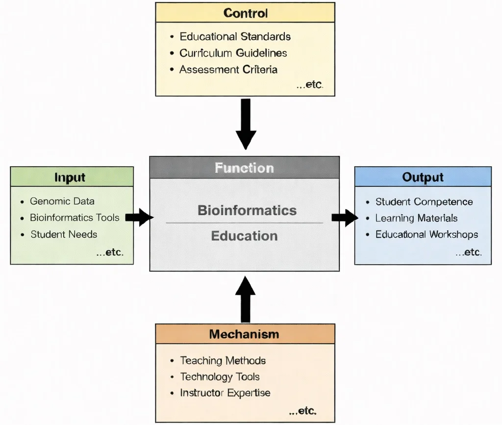
IDEF0 view of Bioinformatics Education: genomic data and bioinformatics tools guided by standards and assessment, enabled by teaching and tools, producing student competence and learning resources.
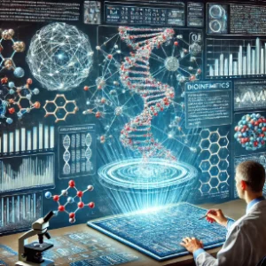
Bioinformatics turns biological data—especially genomes—into insights using computing and analytics. A researcher works at an interactive console while a luminous DNA helix displays molecular structures, sequence alignments, and clinical dashboards.
Biomedical Engineering Cluster Navigation & Knowledge Map
Bioinformatics (Current Page)
Interprets biological complexity by uncovering structural patterns, gene mutations, and metabolic pathways within massive genomic, transcriptomic, and proteomic datasets.
Biomaterials
Reveals interactions at cellular and molecular interfaces, utilizing computational docking and surface chemistry models to ensure tissue compatibility.
Tissue Engineering & Regenerative Medicine
Combines living cells with 3D-printed bio-scaffolds, relying on single-cell sequencing to analyze cellular differentiation and tissue maturation pathways.
Neural Engineering
Captures neural signaling networks, applying machine learning and algorithmic sequence processing to decode brain-computer interface (BCI) inputs.
Cardiovascular Engineering
Integrates hemodynamics with genetic markers to predict vascular remodeling, congenital heart defects, and targeted pharmaceutical interventions.
Biomechanics
Links physical movement and skeletal stress to genetic traits, assisting orthopaedic designers in customizing joint prosthetics to unique patient geometries.
Medical Imaging
Converts radiological scans into multi-dimensional spatial models, intersecting with spatial transcriptomics to map gene activity directly onto anatomical images.
Biomedical Signal Processing
Transforms raw biosensing wave data into clean digital structures suitable for computational genomics and predictive physiological analytics.
Pharmaceutical Engineering
Utilizes virtual drug screening, molecular docking algorithms, and pharmacogenomics to design high-affinity small molecule therapeutics.
Rehabilitation Engineering
Applies genomic and metabolic profiles to tailor adaptive exercise technologies, assistive robotics, and personalized neuromuscular recovery plans.
Clinical Engineering
Integrates bio-computational systems into hospital networks, securing patient genomic databases and point-of-care diagnostic software.
Biomedical Engineering – Overview
Provides the umbrella framework connecting molecular biology, computer science, materials engineering, and clinical device design into a unified discipline.
Core Components of Bioinformatics
Data Acquisition and Storage
- Definition: Systematic collection, curation, and secure warehousing of biological data generated by high-throughput instruments.
- Data Types:
- Genomic Data: Whole-genome DNA/RNA nucleotide sequences from Next-Generation Sequencing (NGS).
- Proteomic Data: Mass spectrometry profiles, amino acid sequences, and protein interaction maps.
- Metabolomic Data: Small molecule metabolite profiles in cellular pathways.
- Primary Databases: NCBI GenBank (nucleotides), Protein Data Bank (3D PDB structures), Ensembl (genomics across species).
Sequence Analysis & Alignment
- Definition: Examining DNA, RNA, and protein sequences to discover functional motifs and evolutionary conservation.
- Key Techniques: Global/Local Sequence Alignment (BLAST, Smith-Waterman), De Novo Genome Assembly, and Automated Gene Annotation.
Data Mining, Machine Learning & Structural Biology
- Data Mining: Clustering gene expressions, predicting disease risk based on single-nucleotide polymorphisms (SNPs), and deep learning models (e.g., AlphaFold for protein folding).
- Structural Bioinformatics: 3D macromolecular modeling, virtual screening, and molecular docking simulations for drug candidate design.
- Systems Biology & Computational Genomics: Integrating multi-omics networks to simulate cell pathways and evaluate whole-genome regulatory mechanisms.
Key Applications of Bioinformatics
- Genomics & Comparative Genomics: Deciphering full DNA codes, tracking disease-causing mutations, and mapping evolutionary relationships across species.
- Drug Discovery & Pharmacogenomics: Identifying high-affinity disease targets, simulating molecular binding, and personalizing drug dosages based on genetic metabolic variations.
- Precision Medicine & Oncology: Tailoring cancer therapies directly to tumor mutational profiles to maximize efficacy while reducing adverse systemic reactions.
- Proteomics & Transcriptomics: Measuring real-time cellular protein levels and RNA transcript dynamics to discover diagnostic bio-markers.
- Metagenomics & Agricultural Genomics: Analyzing environmental microbial communities (human gut microbiome) and enhancing crop yield through genetic marker selection.
Tools and Computational Technologies
- Alignment Tools: BLAST (Basic Local Alignment Search Tool), Clustal Omega (multiple sequence alignment).
- Assembly & Structure Tools: SPAdes (genome assembler), AUGUSTUS (gene prediction), PyMOL (3D visualization), AutoDock (ligand docking).
- Core Languages: Python (BioPython, Pandas), R (Bioconductor), Bash, Perl, and C++ for high-performance computing pipelines.
Challenges & Future Directions
Contemporary AI-Era Computational Paradigms in Bioinformatics
Two homologous genomic sequences of length \(L = 1,000 \text{ base pairs}\) show \(m = 150\) observed nucleotide substitution mismatches, yielding an observed fractional mismatch proportion \(p = \frac{150}{1,000} = 0.150\) (\(15.0\%\)). Due to evolutionary back-mutations and multiple substitutions at identical nucleotide loci over geological epochs, the actual evolutionary divergence distance \(d\) (substitutions per site) exceeds \(p\). Using the Jukes-Cantor one-parameter evolutionary substitution model:
$$d = -\frac{3}{4} \ln\left(1 - \frac{4}{3} p\right)$$Step 1: Compute the inner argument scaling term \(\frac{4}{3} p\):
$$\frac{4}{3} \times 0.150 = 0.200$$Step 2: Evaluate the logarithmic term argument:
$$1 - 0.200 = 0.800$$ $$\ln(0.800) = -0.22314355$$Step 3: Calculate the corrected evolutionary distance \(d\):
$$d = -0.75 \times (-0.22314355) = \mathbf{0.16736 \text{ substitutions/site}}$$Evolutionary Genomics Insight: While direct sequence comparison indicates 15.0% sequence dissimilarity, the Jukes-Cantor correction proves that 16.74 substitutions per 100 sites actually occurred over evolutionary time. This accounts for unobserved hidden transitional reversions, preventing systematic underestimation of phylogenetic branch lengths.
Engineering Trade-offs in Bioinformatics Computing
| Bioinformatics Engineering Trade-off | Primary Computational Benefit | Systemic Penalty / Risk | Quantitative Complexity Metric |
|---|---|---|---|
| Dynamic Programming (Smith-Waterman) vs. Heuristic Search (BLAST) | Guarantees mathematically optimal local sequence alignment with highest sensitivity for divergent sequences. | Quadratic computational complexity; intractable for searching gigabase whole-genome databases. | Time Complexity: Smith-Waterman (\(\mathcal{O}(m \cdot n)\)); BLAST (\(\mathcal{O}(m)\) lookup). |
| Short-Read Sequencing (Illumina) vs. Long-Read Sequencing (Nanopore/PacBio) | Ultra-low base error rate (\(\lt 0.1\%\)) and massive throughput at lowest cost per megabase. | Cannot span repetitive genomic regions, transposons, or complex structural variations (SVs). | Read Length: Short-Read (\(150\text{--}300 \text{ bp}\)); Long-Read (\(10\text{--}100 \text{ kbp}\)). |
| Full All-Atom Molecular Dynamics (MD) vs. Coarse-Grained Virtual Docking | Simulates explicit solvent, conformational entropy, and accurate thermodynamic binding free energies (\(\Delta G\)). | Excessive computational runtime requiring weeks of GPU cluster cluster processing per ligand. | Screening Throughput: Docking (\(10^5 \text{ compounds/day}\)); MD (\(1\text{--}5 \text{ targets/week}\)). |
| High Depth of Sequencing Coverage (\(100\times\)) vs. Standard Depth (\(30\times\)) | Detects ultra-rare sub-clonal cancer mutations, somatic mosaics, and low-frequency viral variants. | Triples sequencing reagent expenditures, data storage footprints, and pipeline processing latency. | Raw Data Output: \(30\times\) Whole Genome (\(\approx 90\text{ GB}\)); \(100\times\) (\(\approx 300\text{ GB}\)). |
In sequence database searching, a raw alignment score \(S\) must be evaluated statistically against the database size to distinguish genuine biological homology from random stochastic sequence matching. The Karlin-Altschul Expectation Value (\(E\)) estimates the number of alignments with a score \(\ge S\) expected purely by chance:
$$E = K \cdot m \cdot n \cdot \exp(-\lambda S)$$For a query sequence length \(m = 400 \text{ bp}\) searched against an international genomic database of effective length \(n = 1.0 \times 10^9 \text{ bp}\), with scoring parameters \(K = 0.10\) and \(\lambda = 0.318\), compare the statistical expectation value for a modest score \(S = 60\) versus an enhanced score \(S = 100\):
Step 1: Compute search space pre-factor \(K \cdot m \cdot n\):
$$K \cdot m \cdot n = 0.10 \times 400 \times (1.0 \times 10^9) = \mathbf{4.0 \times 10^{10} \text{ bp}^2}$$Step 2: Case A - Score \(S = 60\):
$$-\lambda S = -0.318 \times 60 = -19.08$$ $$\exp(-19.08) = 5.1725 \times 10^{-9}$$ $$E_{60} = (4.0 \times 10^{10}) \times (5.1725 \times 10^{-9}) = \mathbf{206.9} \quad (\text{High random false-positive expectation})$$Step 3: Case B - Score \(S = 100\):
$$-\lambda S = -0.318 \times 100 = -31.80$$ $$\exp(-31.80) = 1.5471 \times 10^{-14}$$ $$E_{100} = (4.0 \times 10^{10}) \times (1.5471 \times 10^{-14}) = \mathbf{6.19 \times 10^{-4}} \quad (\text{High statistical confidence of true homology})$$Bioinformatics Interpretation: An E-value of \(6.19 \times 10^{-4}\) indicates there is less than a 1-in-1,600 chance of finding an alignment of this quality in a random sequence database of that size, establishing true evolutionary homology.
Core Mathematical Principles in Bioinformatics
Interactive Tool: Sequence Alignment Identity & Mutation Density Model
Interactive runtime environment: https://prep4uni.online/stem/physical-technologies/biomedical-engineering/bioinformatics/
Interactive Review Questions
1. What is the difference between global and local sequence alignment algorithms?
2. Why are BLOSUM and PAM matrices used in protein sequence alignment?
3. How does Next-Generation Sequencing (NGS) data processing differ from Sanger sequencing?
Frequently Asked Questions on Bioinformatics
What does a bioinformatician actually do day to day?
A bioinformatician spends time cleaning raw sequencing files, running alignment or variant calling pipelines, writing automated scripts (Python/R), visualizing gene clusters, and collaborating with clinical medical teams to interpret genetic results.
Why is bioinformatics so critical in modern healthcare?
Modern genomics generates terabytes of raw DNA data. Without computational tools, this data remains unreadable. Bioinformatics turns raw sequencing reads into actionable clinical insights, revealing disease mutations and drug targets.
How does bioinformatics connect biology with computer science and statistics?
Biological questions drive algorithm design. Sequence alignment algorithms rely on evolutionary mutation assumptions, while differential gene expression analysis uses statistical hypothesis testing to separate true signals from noise.
Is strong biology knowledge more important than strong programming skills?
Both are vital. Software development roles emphasize algorithm efficiency and database design, while research roles require deep understanding of molecular biology and pathway mechanics.
How does bioinformatics assist in cancer diagnosis and treatment?
By comparing healthy and tumor DNA, bioinformaticians identify driver mutations, classify cancer sub-types, predict drug resistance, and recommend targeted therapies for precision oncology.
What programming languages are most widely used in bioinformatics?
Python and R are dominant for data processing, Bioconductor packages, and statistical plotting. Shell scripting (Bash) manages command-line pipelines, while C++ handles core alignment speeds.
How can a student begin learning bioinformatics independently?
Students can start by learning basic Python or R, exploring publicly available genomic datasets on NCBI or Ensembl, and running open-source sequence alignment tools like BLAST.
🎯 Career Guidance Tool Is Bioinformatics Right For You?Explore computational biology pathways, skills assessments, and degree options — before you apply. Interactive Portal: https://prep4uni.online/not-sure-which-field-to-study/?field=biomedical-engineering | Explore Careers → |
Comprehensive Practice Modules in Bioinformatics
Section 1: Foundational Concepts (Review Questions)
1. What is bioinformatics, and why is it defined as an interdisciplinary field?
2. Which core disciplines unite in bioinformatics, and what does each contribute?
3. List three major public biological databases and state their primary data types.
4. How does bioinformatics support Next-Generation Sequencing (NGS) workflows?
5. What is pharmacogenomics, and how does it advance precision healthcare?
6. Explain the difference between functional genomics and structural bioinformatics.
7. Why are statistical models essential when processing high-throughput omics data?
8. What is metagenomics, and what health applications does it support?
9. How do multiple sequence alignment tools (e.g., Clustal Omega) assist evolutionary biology?
10. What is the role of guide RNA design algorithms in CRISPR gene editing?
Section 2: Analytical & Scenario-Based Analysis
1. How has Next-Generation Sequencing (NGS) transformed bioinformatics, and what computational bottlenecks have emerged?
2. In personalized oncology, how do bioinformaticians identify driver mutations versus passenger mutations in a tumor sample?
3. What are the limitations of relying purely on virtual molecular docking for initial drug candidate screening?
4. How do machine learning algorithms handle high-dimensional gene expression data without overfitting?
5. Why is single-cell RNA sequencing (scRNA-seq) superior to traditional bulk RNA sequencing for studying tumor heterogeneity?
6. Discuss the ethical concerns surrounding open-access deposition of human genomic data.
7. How does multi-omics data integration improve disease pathway modeling compared to single-layer genomics?
8. An alignment algorithm fails to map short reads across a repetitive genomic region. What strategy resolves this assembly ambiguity?
Section 3: Quantitative Numerical Problems with Step-by-Step Solutions
1. Jukes-Cantor Evolutionary Substitution Distance Calculation
Problem: Two aligned homologous DNA sequences show a proportion of mismatched nucleotides \(p = 0.150\) (\(15.0\%\) difference). Calculate the evolutionary substitution distance \(d\) per site using the Jukes-Cantor model.
Answer:
Step 1: State the Jukes-Cantor formula:
\(d = -\frac{3}{4} \ln\left(1 - \frac{4}{3} p\right)\)
Step 2: Compute scaling factor \(\frac{4}{3} p\):
\(\frac{4}{3} \times 0.150 = 0.200\)
Step 3: Evaluate natural logarithm:
\(1 - 0.200 = 0.800 \Rightarrow \ln(0.800) \approx -0.22314\)
Step 4: Compute evolutionary distance \(d\):
\(d = -0.75 \times (-0.22314) = \mathbf{0.1674 \text{ substitutions/site}}\)
The corrected evolutionary distance is 0.1674 substitutions/site.
2. Shannon Entropy of a Multiple Sequence Alignment Column
Problem: In a multiple sequence alignment column of 8 sequences, 6 contain Adenine ('A') and 2 contain Guanine ('G'). Calculate the Shannon Entropy \(H\) (in bits) for this alignment position.
Answer:
Step 1: Compute nucleotide relative frequencies:
\(p_A = \frac{6}{8} = 0.750, \quad p_G = \frac{2}{8} = 0.250\)
Step 2: Evaluate base-2 logarithms (\(\log_2(x) = \frac{\ln(x)}{\ln(2)}\)):
\(\log_2(0.750) \approx -0.41504, \quad \log_2(0.250) = -2.000\)
Step 3: Calculate individual entropy terms (\(p_i \log_2(p_i)\)):
\(p_A \log_2(p_A) = 0.750 \times (-0.41504) = -0.31128\)
\(p_G \log_2(p_G) = 0.250 \times (-2.000) = -0.5000\)
Step 4: Sum and negate terms (\(H = -\sum p_i \log_2(p_i)\)):
\(H = -(-0.31128 - 0.5000) = -(-0.81128) = \mathbf{0.811 \text{ bits}}\)
The alignment column Shannon entropy is 0.811 bits.
3. BLAST Search Expectation Value (E-Value) Calculation
Problem: Calculate the BLAST Expectation Value (\(E\)-value) for a query length \(m = 400 \text{ bp}\) searched against a database size \(n = 1.0 \times 10^9 \text{ bp}\), given scoring constants \(K = 0.10\), \(\lambda = 0.318\), and a raw alignment score \(S = 100\).
Answer:
Step 1: Compute search space pre-factor (\(K \cdot m \cdot n\)):
\(K \cdot m \cdot n = 0.10 \times 400 \times (1.0 \times 10^9) = 4.0 \times 10^{10}\)
Step 2: Compute exponential decay factor (\(\exp(-\lambda S)\)):
-\lambda S = -0.318 \times 100 = -31.80
\(\exp(-31.80) \approx 1.5471 \times 10^{-14}\)
Step 3: Multiply factors (\(E = (K \cdot m \cdot n) \times \exp(-\lambda S)\)):
\(E = (4.0 \times 10^{10}) \times (1.5471 \times 10^{-14}) = \mathbf{6.19 \times 10^{-4}}\)
The BLAST \(E\)-value is 6.19 × 10⁻⁴.
4. Genomic Sequence GC Content Percentage Calculation
Problem: A DNA sequence of \(1,500 \text{ bp}\) contains \(420\) Guanine ('G') and \(380\) Cytosine ('C') bases. Calculate the GC content percentage of the sequence.
Answer:
Step 1: Sum G and C base counts:
\(G + C = 420 + 380 = 800 \text{ bp}\)
Step 2: Compute GC content percentage (\(\text{GC\%} = \frac{G + C}{\text{Total Length}} \times 100\)):
\(\text{GC\%} = \left(\frac{800}{1,500}\right) \times 100 = \mathbf{53.33\%}\)
The sequence has a GC content of 53.33%.
5. Needleman-Wunsch Global Dynamic Sequence Alignment Score
Problem: Compute the global alignment score between two 10-bp sequences using Needleman-Wunsch parameters: Match = \(+2\), Mismatch = \(-1\), Gap Penalty = \(-2\). The alignment yields 7 matches, 1 mismatch, and 2 gaps.
Answer:
Step 1: Formulate scoring equation:
\(\text{Score} = (\text{Matches} \times 2) + (\text{Mismatches} \times -1) + (\text{Gaps} \times -2)\)
Step 2: Calculate individual score contributions:
\(\text{Match Score} = 7 \times (+2) = +14\)
\(\text{Mismatch Penalty} = 1 \times (-1) = -1\)
\(\text{Gap Penalty} = 2 \times (-2) = -4\)
Step 3: Sum contributions:
\(\text{Total Score} = +14 - 1 - 4 = \mathbf{+9}\)
The final Needleman-Wunsch alignment score is +9.
6. RNA-Seq Differential Expression Log2 Fold Change
Problem: In an RNA-seq differential expression experiment, Gene X shows an expression level of \(256 \text{ RPKM}\) in drug-treated cells and \(16 \text{ RPKM}\) in control cells. Calculate the \(\log_2\) fold change.
Answer:
Step 1: Compute raw fold change ratio:
\(\text{Fold Ratio} = \frac{\text{Treated}}{\text{Control}} = \frac{256}{16} = 16.0\)
Step 2: Evaluate base-2 logarithm (\(\log_2(16.0)\)):
\(\log_2(16.0) = \mathbf{+4.00}\)
Gene X exhibits a +4.0 log₂ fold increase (representing a 16-fold upregulation).
7. Whole-Genome NGS Sequencing Total Read Count Calculation
Problem: A whole-human-genome sequencing project (\(G = 3.20 \times 10^9 \text{ bp}\)) aims for \(C = 30\times\) depth of coverage. If short reads have length \(L = 150 \text{ bp}\), calculate the total number of sequencing reads (\(N\)) required.
Answer:
Step 1: Apply Lander-Waterman coverage formula (\(C = \frac{N \cdot L}{G}\)):
\(N = \frac{C \cdot G}{L}\)
Step 2: Calculate total nucleotide throughput needed:
\(\text{Total Bases} = 30 \times (3.20 \times 10^9 \text{ bp}) = 9.60 \times 10^{10} \text{ bp}\)
Step 3: Divide by read length to solve for read count (\(N\)):
\(N = \frac{9.60 \times 10^{10} \text{ bp}}{150 \text{ bp/read}} = \mathbf{6.40 \times 10^8 \text{ reads}}\) (\(640 \text{ million reads}\))
The experiment requires 6.40 × 10⁸ reads (640 million reads).