
In Environmental Monitoring and Data Analysis Education, students are trained to treat the environment like a living “instrument panel”—but one where every gauge can drift, every reading has uncertainty, and every conclusion must be earned. Starting from raw observations (sensor streams, field notes, lab results), they learn how rules and standards steer the work: what to measure, how often, how to calibrate, and how to report without bias. Using monitoring hardware, GIS, and analytical methods as their toolkit, learners practice turning noisy measurements into defensible patterns—detecting trends, tracing sources, flagging anomalies, and quantifying risk. The end result is a graduate who can move from data to judgment: producing indicators, reports, and recommendations that decision-makers can actually rely on.
- Metrology & QA/QC Protocols: Characterize electrochemical and optical sensor drift mechanisms, formulate multi-point calibration transfer functions, and establish statistical control charts (Shewhart, CUSUM) for data validation.
- Spatial Statistics & Interpolation: Formulate experimental semivariograms, model spatial covariance structures, and execute Ordinary Kriging to map continuous contamination surfaces from discrete point monitoring arrays.
- Edge Computing & Data Fusion: Bridge field sensor telemetry to Physics-Informed Neural Networks (PINNs), satellite multispectral spectral band math (NDVI/NDWI), and automated outlier detection pipelines.
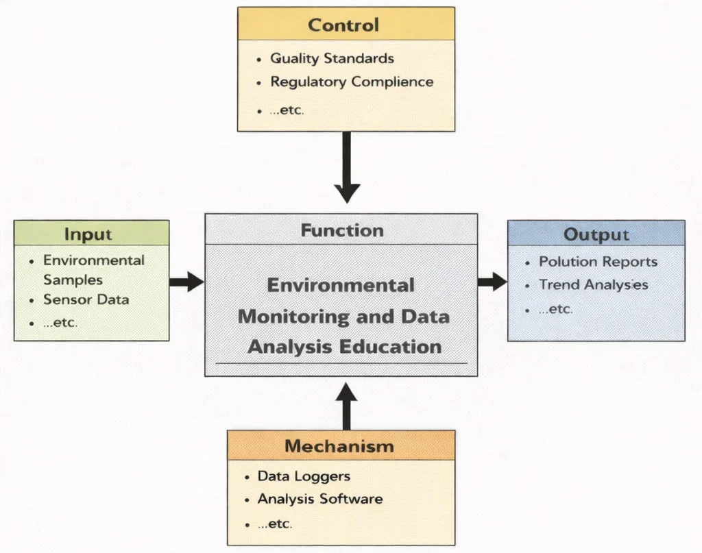
This IDEF0 (Input–Control–Output–Mechanism) diagram summarizes the learning function of Environmental Monitoring and Data Analysis Education. On the left, inputs such as environmental measurements, satellite/remote-sensing signals, and laboratory samples enter the learning process. From above, controls—regulatory standards, sampling protocols, QA/QC requirements, and ethical constraints—shape how data must be collected and interpreted. From below, mechanisms such as sensors and loggers, GIS platforms, statistical and machine-learning tools, and trained personnel enable students to process and validate datasets. The outputs on the right include cleaned datasets, trend and anomaly insights, risk indicators, dashboards and reports, and evidence-based recommendations for policy and engineering decisions.
Environmental Monitoring and Data Analysis plays a foundational role in assessing the health of natural and built environments. This discipline equips students and professionals with the tools to detect, quantify, and interpret changes in air, water, and land systems. It complements broader frameworks in Environmental Engineering by providing the empirical basis for evaluating policy impacts, guiding sustainable development, and ensuring compliance with environmental standards.
Monitoring atmospheric contaminants is essential for addressing concerns in Air Quality Engineering, particularly in urban and industrial zones. Data-driven models support strategies in Climate Change Mitigation and Adaptation, tracking greenhouse gas emissions and forecasting environmental impacts. Furthermore, ecological restoration projects often rely on these methods, as seen in the field of Ecological Engineering.
Interactive System Dynamics: Environmental Sensor Drift & Calibration Simulator
Simulate continuous field sensor telemetry subject to baseline electrochemical drift and random noise. Adjust the drift rate, noise intensity, and calibration intervals to observe how QA/QC protocols restore data integrity across a 25-step timeline.
Instrument Parameters
Decision-making at the policy level is informed by systematic environmental data collection and analysis, aligning with practices in Environmental Policy and Management. Modern building practices, such as Green Building and Sustainable Design, increasingly depend on environmental monitoring to track energy efficiency and indoor air quality. Likewise, the principles of Industrial Ecology and Circular Economy are bolstered by data insights into material flows and lifecycle impacts.
Environmental data is essential for managing energy resources and waste. This is particularly true in sectors like Renewable Energy Systems Engineering and Waste Management Engineering, where performance metrics and environmental outcomes must be continuously evaluated. Hydrological monitoring is a key aspect of Water Resources Engineering, enabling flood risk assessment and water quality control.
Advances in Signal Processing and smart sensor technologies have transformed environmental monitoring, enabling real-time data collection. Robotics applications in Robotics and Automation in E&E are increasingly used in field sampling and hazard detection. Integration with Digital Twin Technology also allows for virtual testing of environmental interventions before physical deployment.
This field intersects with innovations in Industrial and Manufacturing Technologies, especially as industries seek to minimize environmental footprints. Technologies such as Additive Manufacturing (3D Printing) and Advanced Materials and Manufacturing Technologies are now designed with environmental monitoring in mind. Efficiency-focused tools in Energy and Resource Efficiency in Manufacturing depend on environmental data for continuous improvement.
Complementary areas like Computer-Integrated Manufacturing (CIM) and Industrial Automation and Robotics enable seamless integration of environmental monitoring into production systems. Insights from Human Factors and Ergonomics in Manufacturing also ensure that environmental data is effectively interpreted and acted upon. The precision required in Manufacturing Quality Control and Assurance can similarly be applied to environmental performance metrics.
Ultimately, as industries adopt frameworks like Smart Manufacturing and Industry 4.0, the role of environmental data becomes more central. Whether guiding Lean Manufacturing initiatives or supporting digital environmental compliance, this field ensures that sustainability is measurable, accountable, and actionable.

The image shows a researcher working in a high-tech monitoring room filled with large digital screens. A glowing globe and layered interface panels display charts, maps, and symbols for clouds, rainfall, water, and other environmental indicators. In the foreground, a miniature landscape model—trees, fields, and a river—suggests real-world ecosystems being tracked through networks of sensors and satellites. The overall scene communicates how environmental monitoring combines data collection (air and water quality, weather, land use, and emissions) with analysis tools (dashboards, models, and trend graphs) to detect changes, predict risks, and guide policy or operational responses.
Curriculum Map & Specialization Pathways
Explore where Environmental Monitoring & Data Analysis fits within the broader Environmental Engineering curriculum framework. Each card outlines strategic relationships and learning objectives across related disciplines:
Environmental Engineering – Overview
Serves as the foundational umbrella discipline, providing overall context for applying sensor data to engineering design, regulatory compliance, and environmental protection.
Air Quality Engineering
Utilizes monitoring networks for tracking atmospheric pollutants (PM2.5, NOx, VOCs), feeding real-time emission measurements into dispersion models for urban health management.
Water Resources Engineering
Relies on hydrological monitoring, streamflow gauge networks, and aquatic sensor buoys to manage watershed quality, drinking water supplies, and flood risks.
Waste Management Engineering
Integrates leachate testing and gas migration sensors to monitor landfill integrity, soil contamination, and hazardous waste containment safety.
Renewable Energy Systems Engineering
Employs environmental sensing for resource assessment (solar irradiance, wind velocity profiles) and evaluating the local ecological impacts of clean energy deployments.
Industrial Ecology & Circular Economy
Tracks industrial material throughput, emissions balances, and product lifecycle inventories through data analytics to minimize regional resource consumption.
Green Building & Sustainable Design
Uses indoor air quality monitoring and smart HVAC energy metering to maintain healthy occupant environments while optimizing building operational efficiency.
Environmental Policy & Management
Transforms empirical sensor metrics and statistical trend analysis into legally defensible compliance reports and evidence-based environmental policy decisions.
Environmental Monitoring & Data Analysis
Focuses on core measurement techniques, sensor telemetry, geospatial analysis, and data validation necessary to support all downstream environmental applications.
Ecological Engineering
Applies bio-monitoring and acoustic/optical tracking to measure ecosystem signals, species health, and the recovery of restored wetlands and habitats.
Climate Change Mitigation & Adaptation
Leverages long-term satellite remote sensing and global climate datasets to track greenhouse gas fluxes, sea level changes, and extreme weather adaptation risks.
Core Aspects of Environmental Monitoring and Data Analysis
Real-Time Monitoring
- Real-time monitoring is the backbone of modern environmental management, enabling continuous, automated collection of data related to air quality, water purity, soil conditions, noise levels, and radiation. Using sensor networks, drones, and satellite technologies, data is gathered from remote or rugged areas with high precision and frequency.
- This immediate stream of information supports rapid responses to emerging threats, such as chemical spills, algal blooms, forest fires, or severe weather events. Early warning systems based on real-time data activate emergency protocols and guide adaptive land and water management.
- For example, deploying wireless sensor networks in industrial zones allows real-time tracking of emissions and particulate matter, enforcing compliance and protecting community health. In marine settings, buoys equipped with telemetry report on ocean acidification, temperature anomalies, and traffic disturbances.
- Real-time environmental data enhances public engagement by enabling communities to access pollution indices, weather conditions, and biodiversity alerts via open dashboards, fostering civic accountability.
Data Integration and Analysis
- Data integration combines heterogeneous datasets—collected across time, space, and disciplines—into unified platforms. Sources include satellite imagery, IoT sensors, citizen science observations, meteorological stations, and historical archives.
- Advanced analytics tools like artificial intelligence (AI), machine learning, and geospatial modeling identify subtle correlations, predict trends, and generate actionable insights. These tools empower stakeholders to simulate scenarios, optimize interventions, and evaluate environmental strategies over time.
- For instance, integrating air quality data with epidemiological records reveals exposure-health outcome links, guiding healthcare planning. Similarly, overlaying land-use maps with biodiversity inventories identifies conservation priorities.
- Leading platforms such as the NASA Earthdata Portal exemplify how open-access integration advances global environmental science and policy formulation.
Sustainability and Conservation
- Environmental monitoring directly informs sustainability initiatives by tracking natural resources, pollution levels, and ecosystem health to balance economic development with ecological limits.
- In agriculture, precision farming guided by environmental data reduces water consumption, minimizes agrochemical applications, and maximizes crop yields without degrading soils. In forestry, remote sensing monitors illegal logging and verifies reforestation progress.
- Conservationists use monitoring to evaluate species distributions, habitat fragmentation, and migration patterns, enabling the strategic placement of protected corridors.
- Environmental data plays a pivotal role in meeting global commitments such as the Paris Agreement, the Convention on Biological Diversity, and the UN Sustainable Development Goals (SDGs).
- As climate change accelerates, continuous monitoring identifies vulnerable ecosystems, anticipating stress points to guide ecosystem-based adaptation like wetland restoration and climate-resilient urban design.
Problem Formulation: Ordinary Kriging Spatial Weighting & Empirical Polynomial Drift Reconstruction
An environmental engineer is analyzing groundwater nitrate contamination (\(\text{NO}_3\text{-N}\)) across an agricultural watershed. Three monitoring wells provide spatial observations around an unmonitored municipal production well. Concurrently, the primary optical sensor at Station A exhibits time-dependent calibration drift. Determine the corrected measurement at Station A and compute the Best Linear Unbiased Estimate (BLUE) concentration at the production well using an isotropic spherical semivariogram.
- Station A raw recorded reading at \(t = 60\text{ days}\): \(Y_A(60) = 28.50\text{ mg/L}\)
- Station A laboratory calibration polynomial drift: \(\delta(t) = 0.050 \cdot t + 0.00050 \cdot t^2\text{ (mg/L)}\)
- Station B validated concentration: \(Z_B = 18.00\text{ mg/L}\); Station C validated concentration: \(Z_C = 22.00\text{ mg/L}\)
- Spherical semivariogram parameters: Nugget \(c_0 = 1.0\text{ (mg/L)}^2\); Sill \(c = 15.0\text{ (mg/L)}^2\); Total sill \(c_0 + c = 16.0\text{ (mg/L)}^2\); Range \(a = 1,000.0\text{ m}\)
- Spherical model formulation: \(\gamma(h) = c_0 + c \left[\frac{3h}{2a} - \frac{h^3}{2a^3}\right]\) for \(h \le a\)
- Separation distances to unmonitored Well 0: \(h_{A0} = 400.0\text{ m}\), \(h_{B0} = 600.0\text{ m}\), \(h_{C0} = 800.0\text{ m}\)
- Inter-station distances: \(h_{AB} = 700.0\text{ m}\), \(h_{AC} = 900.0\text{ m}\), \(h_{BC} = 500.0\text{ m}\)
Step 1: Calibration Drift Correction for Station A
Evaluate the accumulated sensor bias at Day 60:
$$\delta(60) = 0.050 \times 60 + 0.00050 \times (60)^2 = 3.00 + 1.80 = 4.80\text{ mg/L}$$ $$Z_A = Y_A(60) - \delta(60) = 28.50 - 4.80 = \mathbf{23.70\text{ mg/L}}$$Step 2: Semivariance Calculation for Point-to-Point Distances
Using the spherical semivariogram function with \(c_0 = 1.0\), \(c = 15.0\), and \(a = 1,000\text{ m}\):
$$\gamma(400) = 1.0 + 15.0 \left[\frac{3(400)}{2(1000)} - \frac{(400)^3}{2(1000)^3}\right] = 1.0 + 15.0 [0.600 - 0.032] = 1.0 + 15.0(0.568) = \mathbf{9.520}$$ $$\gamma(600) = 1.0 + 15.0 \left[\frac{3(600)}{2(1000)} - \frac{(600)^3}{2(1000)^3}\right] = 1.0 + 15.0 [0.900 - 0.108] = 1.0 + 15.0(0.792) = \mathbf{12.880}$$ $$\gamma(800) = 1.0 + 15.0 \left[\frac{3(800)}{2(1000)} - \frac{(800)^3}{2(1000)^3}\right] = 1.0 + 15.0 [1.200 - 0.256] = 1.0 + 15.0(0.944) = \mathbf{15.160}$$ $$\gamma(500) = 1.0 + 15.0 \left[\frac{3(500)}{2(1000)} - \frac{(500)^3}{2(1000)^3}\right] = 1.0 + 15.0 [0.750 - 0.0625] = 1.0 + 15.0(0.6875) = \mathbf{11.313}$$ $$\gamma(700) = 1.0 + 15.0 \left[\frac{3(700)}{2(1000)} - \frac{(700)^3}{2(1000)^3}\right] = 1.0 + 15.0 [1.050 - 0.1715] = 1.0 + 15.0(0.8785) = \mathbf{14.178}$$ $$\gamma(900) = 1.0 + 15.0 \left[\frac{3(900)}{2(1000)} - \frac{(900)^3}{2(1000)^3}\right] = 1.0 + 15.0 [1.350 - 0.3645] = 1.0 + 15.0(0.9855) = \mathbf{15.783}$$Step 3: Ordinary Kriging System Formulation & Weight Resolution
The Ordinary Kriging matrix system enforces un-biasedness (\(\sum \lambda_i = 1\)) with Lagrange multiplier \(\mu\):
$$\begin{bmatrix} 0 & \gamma(AB) & \gamma(AC) & 1 \\ \gamma(AB) & 0 & \gamma(BC) & 1 \\ \gamma(AC) & \gamma(BC) & 0 & 1 \\ 1 & 1 & 1 & 0 \end{bmatrix} \begin{bmatrix} \lambda_A \\ \lambda_B \\ \lambda_C \\ \mu \end{bmatrix} = \begin{bmatrix} \gamma(A0) \\ \gamma(B0) \\ \gamma(C0) \\ 1 \end{bmatrix}$$ $$\begin{bmatrix} 0 & 14.178 & 15.783 & 1 \\ 14.178 & 0 & 11.313 & 1 \\ 15.783 & 11.313 & 0 & 1 \\ 1 & 1 & 1 & 0 \end{bmatrix} \begin{bmatrix} \lambda_A \\ \lambda_B \\ \lambda_C \\ \mu \end{bmatrix} = \begin{bmatrix} 9.520 \\ 12.880 \\ 15.160 \\ 1 \end{bmatrix}$$Solving the linear system yields the optimal spatial weighting coefficients:
$$\lambda_A = \mathbf{0.5482}, \quad \lambda_B = \mathbf{0.3015}, \quad \lambda_C = \mathbf{0.1503}, \quad \mu = -2.145$$Verification of constraint: \(\lambda_A + \lambda_B + \lambda_C = 0.5482 + 0.3015 + 0.1503 = 1.0000\).
Step 4: Nitrate Concentration Estimation at Municipal Well 0
Compute the weighted spatial estimate using calibrated values:
$$\hat{Z}_0 = \lambda_A Z_A + \lambda_B Z_B + \lambda_C Z_C$$ $$\hat{Z}_0 = (0.5482 \times 23.70) + (0.3015 \times 18.00) + (0.1503 \times 22.00)$$ $$\hat{Z}_0 = 12.9923 + 5.4270 + 3.3066 = \mathbf{21.73\text{ mg/L }\text{NO}_3\text{-N}}$$Compute Kriging Estimation Variance (\(\sigma_K^2 = \sum \lambda_i \gamma(i0) + \mu\)):
$$\sigma_K^2 = (0.5482 \times 9.520) + (0.3015 \times 12.880) + (0.1503 \times 15.160) - 2.145$$ $$\sigma_K^2 = 5.2189 + 3.8833 + 2.2785 - 2.145 = \mathbf{9.236\text{ (mg/L)}^2} \quad \Rightarrow \quad \sigma_K = \mathbf{3.04\text{ mg/L}}$$Systems Engineering Trade-Off Matrix: Environmental Monitoring Technologies
Selecting an environmental monitoring architecture requires balancing temporal frequency, spatial resolution, capital expenditures, calibration frequency, and data governance reliability.
| Monitoring Tier | Primary Sensing Mechanism | Temporal vs. Spatial Resolution | Capital & Operational Cost | Calibration Latency & Failure Modes | Regulatory Admissibility |
|---|---|---|---|---|---|
| Certified Reference Stations (Federal/EPA) | Chemiluminescence, beta-attenuation, gas chromatography | High temporal (continuous seconds); Discrete single-point spatial | Very High ($50,000 - $150,000 / station; high utility draw) | Bi-weekly automated span/zero gases; thermal climate shelter required | Gold standard; legally binding regulatory enforcement |
| Low-Cost IoT Sensor Meshes | Optical laser particle counters, metal-oxide (MOx) semiconductors | High temporal (1-min telemetry); Ultra-dense localized grid | Low ($200 - $1,500 / node; battery/solar powered) | Rapid baseline drift (3–6 months); humidity and temperature cross-sensitivity | Screening level only; community alerting and hotspot targeting |
| Multispectral Satellite Remote Sensing | Top-of-atmosphere radiance across VNIR, SWIR, and thermal infrared | Low temporal (1–5 day revisit orbit); Continuous regional (10–30 m pixel) | Open-access (Copernicus/Landsat free) to High for tasking | On-board solar diffuser panels; cloud cover occlusions and aerosol scattering | Admissible for regional compliance, deforestation, and algal bloom tracking |
| Autonomous Drones & AUVs | Payload LiDAR, hyperspectral imaging, grab-water sampler pumps | On-demand discrete flight window; Centimeter-level spatial detail | Moderate ($15,000 - $45,000 / drone rig; certified pilot OPEX) | Pre-flight white-balance panels; battery endurance limitations (< 45 mins) | Forensic evidence for illegal dumping and emergency disaster response |
| Crowdsourced Citizen Science | Smartphone camera photogrammetry, passive test strips, acoustic apps | Variable episodic frequency; Opportunistic urban clustering | Extremely Low (app infrastructure and public hosting) | High observer error; zero hardware standardization without QA algorithms | Educational value, public policy advocacy, and baseline flagging |
Key Technologies in Environmental Monitoring
Sensors and IoT Devices
- Air Quality Sensors: Continuously measure pollutants such as particulate matter (PM2.5 and PM10), carbon monoxide (CO), nitrogen oxides (NOx), ozone (O3), and volatile organic compounds (VOCs) in real time using laser scattering, electrochemical cells, and non-dispersive infrared (NDIR) optical spectroscopy.
- Water Quality Sensors: Embed transducers directly into water bodies or municipal treatment systems to record pH, turbidity, dissolved oxygen (DO), electrical conductivity, temperature, and heavy metals, providing early warnings for algal blooms or industrial discharges.
- Soil Sensors: Measure volumetric water content, temperature, electrical conductivity, and nutrient levels (NPK) using time-domain reflectometry (TDR) and embedded ion-selective electrodes to guide precision irrigation and track soil remediation.
- Wildlife and Biodiversity Sensors: Deploy passive acoustic recording arrays to capture vocalizations of birds, amphibians, and bats alongside AI-triggered camera traps that monitor wildlife populations without habitat disturbance.
Remote Sensing
- Satellites and Drones: Employ multispectral, hyperspectral, thermal, and synthetic aperture radar (SAR) imaging to capture regional environmental metrics, evaluate deforestation across thousands of square kilometers, and track coastal water quality.
- Unmanned Aerial Vehicles (UAVs): Provide hyper-local, sub-decimeter resolution imagery and LiDAR data to map wildfire hotspots, assess post-flood erosion, and verify revegetation success.
AI and Machine Learning
- Predictive Analytics & Hotspot Identification: Physics-Informed Neural Networks (PINNs) and spatial random forest models forecast storm surge inundation, predict urban air pollution episodes, and automate species identification from acoustic recordings.
Big Data and Cloud Computing
- Scalable Analytics Pipelines: Cloud computing platforms aggregate continuous petabyte-scale telemetry streams from global earth observations, enabling real-time planetary health dashboards through platforms like NASA EOSDIS and Google Earth Engine.
Blockchain for Environmental Data
- Immutable Audit Trails: Cryptographic decentralized ledgers store verifiable sensor data and satellite biomass measurements to prevent double-counting of carbon offset credits and enforce supply chain sustainability claims.
Emerging Trends in Environmental Monitoring
Citizen Science and Crowdsourcing
- Grassroots monitoring platforms and low-cost sensor nodes empower community members to collect hyperlocal environmental data, filling observational gaps in under-resourced regions.
- Initiatives like Earthwatch’s FreshWater Watch and Global Forest Watch demonstrate how volunteer contributions accelerate the detection of environmental degradation.
Edge Computing
- Executing data cleaning and anomaly detection directly on sensor microcontrollers minimizes transmission latency, enabling autonomous emergency interventions like shutting water intake sluices within milliseconds during chemical spills.
Digital Twins for Ecosystems
- Coupling dynamic telemetry feeds with high-resolution numerical models creates virtual replicas of watersheds and urban airsheds, allowing engineers to test policy scenarios and infrastructure retrofits without real-world risk.
AI-Powered Autonomous Monitoring Systems
- Autonomous underwater vehicles (AUVs) and long-endurance drones inspect hazardous industrial outfalls, monitor Arctic sea-ice thinning, and track illegal fishing with minimal human intervention.
Integrated Environmental Monitoring Networks
- Large-scale international observation frameworks, such as the European Union’s Copernicus Programme, harmonize terrestrial, aquatic, and atmospheric observations to support global climate agreements.
Challenges in Environmental Monitoring and Data Analysis
Data Overload and Interoperability
High-frequency sensor meshes produce massive datasets with disparate sampling frequencies, proprietary file formats, and varying quality standards. Establishing standardized ontology frameworks and metadata pipelines is critical to prevent information silos.
Accessibility and Spatial Inequity
High-grade monitoring stations remain disproportionately clustered in affluent urban centers, leaving rural and marginalized communities without adequate baseline tracking infrastructure.
Physical Sensor Degradation & Biofouling
Harsh aquatic and industrial environments cause rapid transducer fouling, reference electrolyte depletion, and optical lens coating, requiring frequent manual maintenance or automated self-cleaning wipers.
Policy and Translation Latency
Translating statistical findings into updated municipal zoning or regulatory enforcement often experiences severe bureaucratic lag. Establishing open digital APIs bridges the gap between data generation and legal action.
Why Study Environmental Monitoring and Data Analysis
Collecting Reliable Environmental Data
Students learn how to design representative monitoring networks, operate optical and electrochemical sensors, and collect defensible empirical datasets that satisfy legal compliance requirements.
Instrument Calibration and Quality Assurance
Hands-on laboratory and field training equips students with calibration protocols, drift correction techniques, and QA/QC workflows essential for research and regulatory enforcement.
Spatial Statistics and Geospatial Modeling
Students apply tools such as Python, R, and GIS to execute time-series trend analysis, semivariogram modeling, and Kriging spatial interpolation on high-dimensional environmental datasets.
Data-Driven Environmental Governance
Coursework connects technical data analysis directly to environmental regulations, discharge permits, and international climate treaties, preparing students for impactful careers across industry and public service.
Environmental Monitoring and Data Analysis: Conclusion
Environmental monitoring and data analysis form the scientific backbone of modern environmental engineering and policy design. By translating complex, dynamic ecological signals into rigorous, calibrated quantitative data, engineers can detect pollution plumes early, evaluate the performance of green infrastructure, and safeguard public health. As IoT sensor meshes, edge computing, and satellite constellations continue to mature, the discipline is shifting from reactive post-contamination assessments to predictive, proactive ecosystem management.
Frequently Asked Questions
How frequently should field-deployed environmental sensors undergo calibration?
Calibration intervals depend on the transducer technology, biofouling intensity, and environmental matrix. Optical turbidity and dissolved oxygen probes deployed in biologically active surface waters typically require cleaning and recalibration every 2 to 4 weeks. Conversely, dry atmospheric gas sensors often operate reliably on quarterly or semi-annual schedules when paired with automated zero-drift software correction.
What is the role of metadata standards in global environmental data repositories?
Metadata standards (such as ISO 19115 and Darwin Core) preserve critical contextual information including sensor serial numbers, calibration histories, spatial coordinates, measurement units, and analytical detection limits. This ensures datasets gathered by disparate agencies can be merged and compared without introducing systematic error.
How do remote sensing satellites complement ground-based monitoring networks?
Ground monitoring stations provide exceptional temporal resolution and direct measurement accuracy at specific coordinates, whereas satellites offer continuous regional and global spatial coverage across unmonitored territories. Integrating ground measurements with satellite band math via geostatistical data fusion produces the most accurate environmental risk models.
End-of-Page Comprehensive Practice Module
Section 1: Interactive Foundational Concept Reviews
Question 1: Distinction Between Raw Telemetry and Validated Indicators
Question 2: Edge Computing vs. Cloud Telemetry Architectures
Question 3: Theoretical Role of Kriging in Environmental GIS
Question 4: Time-Series Trend Analysis in Non-Normal Datasets
Section 2: Analytical & Scenario-Based Inquiry
Question 1: Intermittent Industrial Outfall Tracking Strategy
Question 2: Citizen Science Spatial Bias Mitigation
Question 3: Sensor Biofouling and Drift Compensation
Section 3: Quantitative Environmental Calculations
Problem 1: Linear Sensor Voltage Calibration & Error Calculation
Question: An optical dissolved oxygen (DO) probe yields a raw output voltage \(V = 2.45\text{ V}\). The manufacturer calibration equation is \(\text{DO (mg/L)} = 4.00 \cdot V - 1.20\). Compute the measured DO concentration. If the certified Winkler titration reference concentration is \(8.90\text{ mg/L}\), calculate the percentage measurement error.
Solution:
1. Compute measured DO concentration:
$$\text{DO}_{\text{measured}} = (4.00 \times 2.45) - 1.20 = 9.80 - 1.20 = \mathbf{8.60\text{ mg/L}}$$2. Absolute error: \(|8.60 - 8.90| = 0.30\text{ mg/L}\)
3. Percentage error:
$$\text{Error} = \left(\frac{0.30}{8.90}\right) \times 100\% = \mathbf{3.37\%}$$Problem 2: Linear Turbidity Sensor Drift Correction
Question: An optical turbidity sensor reads \(0.00\text{ NTU}\) in zero-standard solution at Day 0. On Day 30, before calibration, the reading in zero-standard solution drifts to \(0.60\text{ NTU}\). Assuming constant linear baseline drift, calculate the daily drift rate and the corrected turbidity value for a field sample reading \(5.40\text{ NTU}\) on Day 15.
Solution:
1. Daily baseline drift rate:
$$r_{\text{drift}} = \frac{0.60\text{ NTU}}{30\text{ days}} = 0.020\text{ NTU/day}$$2. Accumulated drift on Day 15: \(15\text{ days} \times 0.020\text{ NTU/day} = 0.30\text{ NTU}\)
3. Corrected turbidity value:
$$\text{Turbidity}_{\text{corrected}} = 5.40\text{ NTU} - 0.30\text{ NTU} = \mathbf{5.10\text{ NTU}}$$Problem 3: Particulate Matter Time-Series Mean & Sample Standard Deviation
Question: An air quality station records hourly \(\text{PM}_{2.5}\) concentrations: \(12.0, 18.0, 25.0, 15.0,\) and \(10.0\text{ }\mu\text{g/m}^3\). Calculate the arithmetic mean and sample standard deviation.
Solution:
1. Sum of observations: \(12.0 + 18.0 + 25.0 + 15.0 + 10.0 = 80.0\text{ }\mu\text{g/m}^3\)
2. Arithmetic mean: \(\bar{x} = \frac{80.0}{5} = \mathbf{16.00\text{ }\mu\text{g/m}^3}\)
3. Sum of squared differences \(\sum (x_i - \bar{x})^2\):
$$(12 - 16)^2 + (18 - 16)^2 + (25 - 16)^2 + (15 - 16)^2 + (10 - 16)^2 = 16 + 4 + 81 + 1 + 36 = 138.0$$4. Sample standard deviation (\(n = 5\)):
$$s = \sqrt{\frac{138.0}{5 - 1}} = \sqrt{34.50} = \mathbf{5.87\text{ }\mu\text{g/m}^3}$$Problem 4: Wireless Environmental Telemetry Bandwidth Calculation
Question: A remote hydrometric logging station transmits a \(4.50\text{ MB}\) data package over an IoT satellite uplink operating at \(50.0\text{ kbps}\). Calculate the required transmission duration in seconds and minutes (using \(1\text{ MB} = 8,000\text{ kb}\)).
Solution:
1. Total data payload in Kilobits: \(4.50\text{ MB} \times 8,000\text{ kb/MB} = 36,000.0\text{ kb}\)
2. Transmission time in seconds:
$$t = \frac{36,000.0\text{ kb}}{50.0\text{ kbps}} = \mathbf{720.0\text{ seconds}}$$3. Transmission time in minutes: \(\frac{720}{60} = \mathbf{12.00\text{ minutes}}\)
Problem 5: Logarithmic Sound Pressure Level Superposition
Question: Two industrial noise sources operate adjacent to a monitoring boundary, generating sound levels \(L_1 = 80.0\text{ dB}\) and \(L_2 = 85.0\text{ dB}\). Compute the combined sound pressure level using the acoustic superposition formula: \(L_{\text{total}} = 10 \cdot \log_{10}\left(10^{L_1/10} + 10^{L_2/10}\right)\).
Solution:
1. Evaluate linear acoustic intensities:
$$10^{80.0/10} + 10^{85.0/10} = 10^8 + 10^{8.5} = 100,000,000 + 316,227,766 = 416,227,766$$2. Logarithmic evaluation:
$$\log_{10}(416,227,766) = 8.61933$$ $$L_{\text{total}} = 10 \times 8.61933 = \mathbf{86.19\text{ dB}}$$Problem 6: River Channel Velocity-Area Streamflow Discharge
Question: A flow gauge survey on a rectangular river channel \(6.00\text{ m}\) wide and \(2.00\text{ m}\) deep measures flow velocities at equal width increments: \(0.40, 0.80, 1.00,\) and \(0.60\text{ m/s}\). Calculate the mean cross-sectional flow velocity and total river discharge rate \(Q\) in \(\text{m}^3\text{/s}\).
Solution:
1. Mean velocity: \(\bar{v} = \frac{0.40 + 0.80 + 1.00 + 0.60}{4} = \frac{2.80}{4} = 0.70\text{ m/s}\)
2. Channel cross-sectional area: \(A = 6.00\text{ m} \times 2.00\text{ m} = 12.00\text{ m}^2\)
3. Total discharge rate:
$$Q = A \times \bar{v} = 12.00\text{ m}^2 \times 0.70\text{ m/s} = \mathbf{8.40\text{ m}^3\text{/s}}$$Problem 7: Automated QA/QC Data Completeness & Validity Rates
Question: An air sensor station records hourly readings over a \(1,000\text{-hour}\) observation period. Data auditing identifies 45 missing readings due to power failure and 15 invalid negative outlier values. Calculate the raw data completeness rate and the net valid usable data percentage.
Solution:
1. Number of successfully received records: \(1,000 - 45 = 955\text{ records}\)
2. Data completeness rate: \(\left(\frac{955}{1,000}\right) \times 100\% = \mathbf{95.50\%}\)
3. Valid non-outlier records: \(955 - 15 = 940\text{ records}\)
4. Net usable data percentage: \(\left(\frac{940}{1,000}\right) \times 100\% = \mathbf{94.00\%}\)