
The Second Law of Motion stands at the heart of classical physics, describing how the force acting on an object relates to its mass and acceleration. This principle serves as a cornerstone for analyzing mechanical systems and predicting motion in both everyday and extreme environments. Students begin their exploration of this fundamental idea with a solid grounding in Physics and its subfield classical mechanics, which together build the framework for understanding how motion responds to forces.
To deepen their understanding, learners can turn to analytical mechanics, where generalized coordinates and Lagrangians offer powerful tools for solving problems involving the Second Law. Meanwhile, the celestial scale of celestial mechanics reveals how gravitational forces govern planetary motion under Newton’s laws. A bridge to material behavior is offered by continuum mechanics, which integrates the role of force and stress within continuous media. More immediately related are the modules for dynamics and the baseline definition of inertia.
Applied examples often emerge in fluid mechanics, where pressure forces affect fluid flow, and in kinematics, which analyzes motion without regard to cause. When approaching limits near the speed of light, relativistic mechanics modifies Newtonian principles. Within the more specialized realm of rigid body dynamics, torque and angular acceleration are governed by rotational analogs of Newton’s second law. Static scenarios are addressed through statics, while subsequent balance equations emphasize interaction forces. The study of vibrations and oscillations demonstrates how restoring forces produce periodic acceleration in mechanical systems.
Further insights are gained through the study of Electricity & Magnetism, where forces act on charged particles and current-carrying conductors. Concepts of voltage and current in electrical circuits and the interactions described by electrodynamics reflect how Newton’s laws are extended to electromechanical systems. Related fields such as electromagnetic induction and electromagnetic waves illustrate forces that arise from time-varying fields. An understanding of electrostatics and magnetic fields provides a basis for understanding static electric and magnetic forces, while advanced applications in magnetohydrodynamics (MHD) merge fluid and electromagnetic dynamics.
Finally, fields such as magnetostatics and plasma physics explore the nuanced behavior of systems where Newton’s second law interacts with complex field conditions. Mastery of these interrelated concepts equips students with a powerful toolkit for interpreting both natural and engineered systems through the lens of force and acceleration.
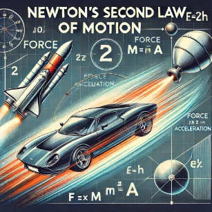
Mathematical Derivation of Newton’s Second Law of Motion
Key Principles of the Formulations:
- Net External Force: Newton’s Second Law applies strictly to the net force vector sum acting on an object, not isolated structural elements. If multiple concurrent loads intersect, they must be added vectorially.
- Inertial Resistance: The mass of an object represents its quantitative scalar resistance to acceleration. A heavier mass requires a proportionally greater force vector to achieve an identical target acceleration rate.
- Directional Alignment: The generated acceleration vector always aligns in the exact same direction as the net external force vector field.
Advanced Dynamics: Variable Mass Distributions
Beyond Constant Mass Systems
- $$\mathbf{F}_{\text{ext}}$$ The net external force vector field acting across the system boundary (e.g., gravity or fluid drag).
- $$\mathbf{v}_{\text{rel}}$$ The relative velocity vector of the escaping or entering mass relative to the main system frame.
- $$\frac{dm}{dt}$$ The time rate of change of the structural mass distribution.
Analytical Bridging: From Force Vectors to Scalar Energy
Deriving the Work-Energy Theorem from the Second Law
The Thermodynamic Coupling of Classical Mechanics
Where Newton’s Second Law Collides with Entropic Arrow of Time
- Mechanical Force Input: The macroscopic work vector field: $$\int \mathbf{F}_{\text{applied}} \cdot d\mathbf{r}$$ introduces organized kinetic energy states into the system boundary.
- Thermal Transition: The damping coefficient $$-c\mathbf{v}$$ represents viscous drag or sliding friction, acting as an energy sink that converts ordered kinetic vectors into chaotic molecular thermal motion.
- Entropic Multiplier: This transition generates local entropy $$\Delta S > 0$$, effectively ensuring that real macro-dynamic systems possess a distinct, irreversible direction in time (the entropic arrow of time).
Numerical Application Examples
Example 1: Pushing a Shopping Cart Layout
Example 2: Braking Dynamics and Transient Deceleration
Example 3: Rocket Propulsion Mechanics
Example 4: Tug-of-War Vector Imbalance
Example 5: Falling Skydiver with Air Fluid Damping
Newton’s Second Law: Interactive Laboratory
Quick Check: Linear Momentum Transitions
Quick Check: Vector Force Imbalances
Why Study the Second Law of Motion
Core Principle of Dynamics
Predicting Motion in Real-World Systems
Vector Representation and Multi-Dimensional Analysis
Experimentation and Verification
Bridge to Broader Mechanics
Second Law of Motion — FAQ
What is the second law of motion?
The second law of motion states that the net external force acting on an object equals the mass of the object multiplied by its acceleration (F = ma). This law provides the quantitative connection between forces and changes in motion.How does the second law differ from the first law?
The first law describes the natural state (constant velocity or rest) when net force is zero. The second law describes how motion changes when a net force acts — namely that the acceleration produced is proportional to the net force and inversely proportional to mass.What does ‘net external force’ mean in the context of the second law?
Net external force refers to the vector sum of all external forces acting on the object. It excludes internal forces or forces internal to a system; only outside forces count. The second law applies only to the net external force.Does the second law apply to objects at rest as well as moving objects?
Yes — the second law applies at any moment, whether the object is at rest or in motion. If the net force is non-zero, the acceleration (which may start from rest) will be non-zero, and the object will begin to accelerate. If net force is zero, motion continues unchanged (constant velocity or rest) in accordance with the first law.Why is mass important in F = ma, and what does it represent?
In F = ma, mass represents the inertia of the object — a measure of how much it resists acceleration under a force. A larger mass requires a larger net force to achieve the same acceleration as a smaller mass.How does the second law relate to free-body diagrams and problem solving?
The second law is central to solving dynamics problems. First you draw a free-body diagram showing all forces acting on the object, then compute the vector sum (net force). By setting F_net = ma along each coordinate axis, you obtain equations of motion that can be solved for acceleration, velocity, or displacement depending on the problem.Does the second law apply to variable mass systems or non-inertial frames?
The classical form F = ma applies directly only to objects of constant mass in inertial frames. For variable mass systems (like rockets ejecting fuel) or non-inertial (accelerating) frames, additional terms (such as momentum flux or fictitious forces) must be considered for correct equations of motion.How does the second law connect to energy and work in mechanics?
When the net force does work on an object, that work changes the object’s kinetic energy. Combining the second law with definitions of work and kinetic energy leads to work–energy theorems: for conservative forces, potential energy plus kinetic energy can remain constant. This energy perspective often simplifies analysis and reveals deep connections between forces, motion, and energy conservation.What are common misconceptions about the second law of motion?
Common misconceptions include thinking that heavier objects always accelerate slower regardless of force applied, forgetting that acceleration is produced by net force, or confusing mass with weight. Another common error is applying F = ma without considering all forces or choosing inconsistent coordinate axes.How can mastering the second law help in physics and engineering problems?
Mastering the second law enables you to analyze a broad range of physical problems — from simple block-and-pulley systems to complex multi-body dynamics, rotational motion, fluid drag, and oscillations. It builds a foundation for designing mechanical systems, analysing motion in robotics and vehicles, and understanding wave motion, vibrations, and more advanced topics.Conclusion on Newton’s Second Law of Motion
Newton’s Second Law of Motion: Review Questions and Answers
- What does Newton’s Second Law of Motion state?Answer: Newton’s Second Law states that the net force acting on an object is equal to the product of its mass and its acceleration, mathematically expressed as $$F = ma$$
- How does mass influence an object’s acceleration when a force is applied?Answer: For a given force, an object with greater mass will experience a smaller acceleration, while a lighter object will accelerate more, demonstrating that acceleration is inversely proportional to mass.
- What is meant by net force?Answer: Net force is the vector sum of all the forces acting on an object. It is the total force that determines the acceleration of the object.
- How can Newton’s Second Law be applied to calculate acceleration?Answer: Acceleration can be calculated by rearranging the equation to: $$a = \frac{F_{\text{net}}}{m}$$ where Fnet is the net force acting on the object and m is its mass.
- In what way does direction play a role in Newton’s Second Law?Answer: Since force and acceleration are vectors, both magnitude and direction are crucial. The direction of the net force determines the direction of the acceleration.
- How is the concept of inertia related to the Second Law?Answer: Inertia is an object’s resistance to changes in its state of motion. Newton’s Second Law quantifies this by showing that a larger mass, which has more inertia, requires a greater force to achieve the same acceleration.
- How do external forces, such as friction, affect the net force in Newton’s Second Law?Answer: External forces like friction oppose motion and reduce the net force available to accelerate an object. This reduction in net force results in a lower acceleration than would be expected from the applied force alone.
- How can Newton’s Second Law be used to analyze collisions?Answer: In collisions, the Second Law helps calculate the forces during impact by relating the change in momentum (mass times velocity change) over the collision time to the net force experienced by the objects.
- How is impulse related to Newton’s Second Law?Answer: Impulse, defined as the product of force and the time interval over which it acts, equals the change in momentum. This relation is a direct consequence of Newton’s Second Law applied over a finite time period.
- Why is Newton’s Second Law fundamental to engineering and physics?Answer: Newton’s Second Law is essential because it provides a quantitative framework for predicting how objects will move under various forces. This underpins the design and analysis of everything from simple machines to complex vehicles and structures.
Newton’s Second Law of Motion: Thought-Provoking Questions
- How might Newton’s Second Law be modified under relativistic conditions?Answer: At speeds approaching the speed of light, the simple form $$F = ma$$ no longer gives the full classical picture. In relativistic mechanics, force is more generally related to the time derivative of momentum, leading to a more complex relationship between force, mass, velocity, and acceleration.
- Can Newton’s Second Law be derived from more fundamental principles?Answer: Yes, it can be related to the conservation of momentum and the symmetry of space and time. These principles, along with Noether’s theorem, reveal that the laws governing force and acceleration are deeply rooted in the fundamental structure of physical law.
- How does the Second Law help us understand the dynamics of non-inertial reference frames?Answer: In non-inertial frames, fictitious forces, such as centrifugal and Coriolis forces, appear. While the Second Law can still be used, these extra forces must be included to accurately describe the observed acceleration, thereby enriching our understanding of motion in accelerating systems.
- What role does Newton’s Second Law play in the design of modern vehicles and machinery?Answer: The Second Law is critical in engineering design because it allows engineers to calculate the forces required for desired accelerations. This aids in optimizing engine performance, ensuring stability, and designing effective braking and control systems in vehicles and machinery.
- How do measurement uncertainties affect the practical application of Newton’s Second Law?Answer: Measurement uncertainties in force, mass, and acceleration can lead to errors in predicting motion. Understanding and minimizing these uncertainties through precise instrumentation and statistical analysis is essential for reliable application in engineering and scientific experiments.
- How might emerging technologies, such as AI and machine learning, enhance our use of Newton’s Second Law in dynamic systems?Answer: AI and machine learning can process vast amounts of data to optimize models of dynamic systems, predict complex motion patterns, and identify non-linear behaviors that are challenging to model analytically. This can lead to improved designs and more efficient control systems.
- What limitations exist in applying Newton’s Second Law to systems with variable mass, such as rockets?Answer: In systems with variable mass, such as rockets, the standard form $$F = ma$$ must be modified to account for the changing mass. The rocket equation, which considers mass loss due to fuel consumption, provides a more accurate description of acceleration in such systems.
- How does Newton’s Second Law interact with the concept of conservation of energy?Answer: While the Second Law relates force to acceleration, conservation of energy provides a complementary perspective by accounting for work done and energy transformations. Together, they offer a comprehensive picture of how forces influence motion and energy distribution in a system.
- In what ways does Newton’s Second Law underpin the analysis of multi-body systems?Answer: For multi-body systems, the Second Law is applied to each component, and their interactions are analyzed through the vector sum of forces. This allows for the study of complex systems like vehicles, machinery, and even planetary systems where individual motions are interdependent.
- How do frictional and drag forces complicate the application of Newton’s Second Law in real-world scenarios?Answer: Frictional and drag forces are often non-linear and can vary with speed, temperature, and surface conditions. These complexities require empirical models or computational fluid dynamics to accurately predict the net force and resulting acceleration in practical applications.
- Could Newton’s Second Law be considered a universal law, or are there circumstances where it fails?Answer: Newton’s Second Law is highly effective in most everyday situations, but it fails at relativistic speeds and in quantum-scale phenomena where classical mechanics is replaced by relativistic or quantum mechanics. These limitations highlight the need for different models in extreme conditions.
- How might future discoveries in physics challenge or refine our understanding of force and acceleration as described by Newton’s Second Law?Answer: Future discoveries in fields like quantum gravity or high-energy physics could reveal new interactions or modifications to the concept of mass and force. Such breakthroughs might lead to a refined version of the Second Law that integrates classical mechanics with emerging theories of the fundamental forces of nature.
Numerical Problems and Solutions
- Problem: An object experiences a net force of 25 N. Find its acceleration given the tracking variables:$$m = 5 \text{ kg}, \quad F = 25 \text{ N}$$ Solution:Using Newton’s Second Law: $$a = \frac{F}{m} = \frac{25}{5} = 5.0 \text{ m/s}^2$$ Answer: $$5.0 \text{ m/s}^2$$
- Problem: A block is pushed with a force of 80 N on a frictionless surface plane. Find its linear acceleration rate given:$$m = 16 \text{ kg}, \quad F = 80 \text{ N}$$ Solution:Using Newton’s Second Law: $$a = \frac{F}{m} = \frac{80}{16} = 5.0 \text{ m/s}^2$$ Answer: $$5.0 \text{ m/s}^2$$
- Problem: An object accelerates uniformly over a fixed window. Find the required net force given these parameters:$$m = 2 \text{ kg}, \quad v_0 = 4 \text{ m/s}, \quad v_f = 12 \text{ m/s}, \quad t = 4 \text{ s}$$ Solution:First, evaluate the acceleration tracking metric: $$a = \frac{v_f – v_0}{t} = \frac{12 – 4}{4} = \frac{8}{4} = 2.0 \text{ m/s}^2$$Apply Newton’s Second Law to establish the net force field: $$F = m \cdot a = 2 \times 2.0 = 4.0 \text{ Newtons}$$ Answer: $$4.0 \text{ N}$$
- Problem: A mass is pulled forward while a non-conservative boundary friction acts directly opposite to the path. Find the resulting acceleration if the metrics map as:$$m = 10 \text{ kg}, \quad F_{\text{pull}} = 100 \text{ N}, \quad F_{\text{friction}} = 30 \text{ N}$$ Solution:First, sum up the colinear force vectors to determine the net force mismatch: $$F_{\text{net}} = F_{\text{pull}} – F_{\text{friction}} = 100 – 30 = 70 \text{ Newtons}$$Isolate system acceleration: $$a = \frac{F_{\text{net}}}{m} = \frac{70}{10} = 7.0 \text{ m/s}^2$$ Answer: $$7.0 \text{ m/s}^2$$
- Problem: Two opposing horizontal forces act simultaneously along a linear baseline. Find the acceleration vector state given:$$m = 5 \text{ kg}, \quad F_{\text{east}} = 40 \text{ N}, \quad F_{\text{west}} = 15 \text{ N}$$ Solution:Taking East as the positive coordinate reference direction: $$F_{\text{net}} = F_{\text{east}} – F_{\text{west}} = 40 – 15 = 25 \text{ N (East)}$$Calculate the acceleration response: $$a = \frac{F_{\text{net}}}{m} = \frac{25}{5} = 5.0 \text{ m/s}^2$$ Answer: $$5.0 \text{ m/s}^2 \text{ East}$$
- Problem: A moving object slows down uniformly to a complete stop under a resistive force field. Calculate the active net force given:$$m = 50 \text{ kg}, \quad v_0 = 20 \text{ m/s}, \quad v_f = 0 \text{ m/s}, \quad t = 10 \text{ s}$$ Solution:Evaluate the transient deceleration field indicator: $$a = \frac{v_f – v_0}{t} = \frac{0 – 20}{10} = -2.0 \text{ m/s}^2$$Apply the constant mass force equation: $$F = m \cdot a = 50 \times (-2.0) = -100 \text{ Newtons}$$ Answer: $$-100 \text{ N}$$ acting directly opposite to the initial direction vector.
- Problem: A vehicle accelerates uniformly from rest along a test track. Find the required net driving force vector if parameters register as:$$m = 1\,500 \text{ kg}, \quad v_0 = 0 \text{ m/s}, \quad v_f = 30 \text{ m/s}, \quad t = 10 \text{ s}$$ Solution:Determine the uniform kinematic acceleration rate: $$a = \frac{v_f – v_0}{t} = \frac{30 – 0}{10} = 3.0 \text{ m/s}^2$$Evaluate the net force: $$F = m \cdot a = 1\,500 \times 3.0 = 4\,500 \text{ Newtons}$$ Answer: $$4\,500 \text{ N}$$
- Problem: A constant linear force field acts continuously across a short timeline. Find the resulting change in the particle’s velocity profile given:$$m = 2 \text{ kg}, \quad F = 100 \text{ N}, \quad t = 5 \text{ s}$$ Solution:First, track the system acceleration profile: $$a = \frac{F}{m} = \frac{100}{2} = 50.0 \text{ m/s}^2$$Integrate across the time duration to isolate velocity shift: $$\Delta v = a \cdot t = 50.0 \times 5 = 250.0 \text{ m/s}$$ Answer: $$250.0 \text{ m/s}$$
- Problem: Two completely perpendicular force vector fields act simultaneously on a single mass housing element. Find the magnitude and angle direction of the resulting acceleration vector given:$$m = 10 \text{ kg}, \quad F_{\text{east}} = 30 \text{ N}, \quad F_{\text{north}} = 40 \text{ N}$$ Solution:Evaluate the total resultant force field magnitude using vector additions: $$F_{\text{net}} = \sqrt{F_{\text{east}}^2 + F_{\text{north}}^2} = \sqrt{30^2 + 40^2} = \sqrt{900 + 1600} = 50.0 \text{ Newtons}$$Calculate the acceleration magnitude: $$a = \frac{F_{\text{net}}}{m} = \frac{50.0}{10} = 5.0 \text{ m/s}^2$$Isolate the directional tracking angle relative to the East coordinate baseline axis: $$\theta = \tan^{-1}\left(\frac{F_{\text{north}}}{F_{\text{east}}}\right) = \tan^{-1}\left(\frac{40}{30}\right) \approx 53.1^{\circ}$$ Answer: $$5.0 \text{ m/s}^2$$ directed at exactly $$53.1^{\circ} \text{ North of East}$$.
- Problem: A known load force profile creates a measured steady-state linear acceleration rate. Isolate the target system’s inertial scalar mass value:$$F = 25 \text{ N}, \quad a = 2.5 \text{ m/s}^2$$ Solution:Rearranging Newton’s Second Law to solve for mass variables: $$m = \frac{F}{a}$$ $$m = \frac{25}{2.5} = 10.0 \text{ kg}$$ Answer: $$10.0 \text{ kg}$$