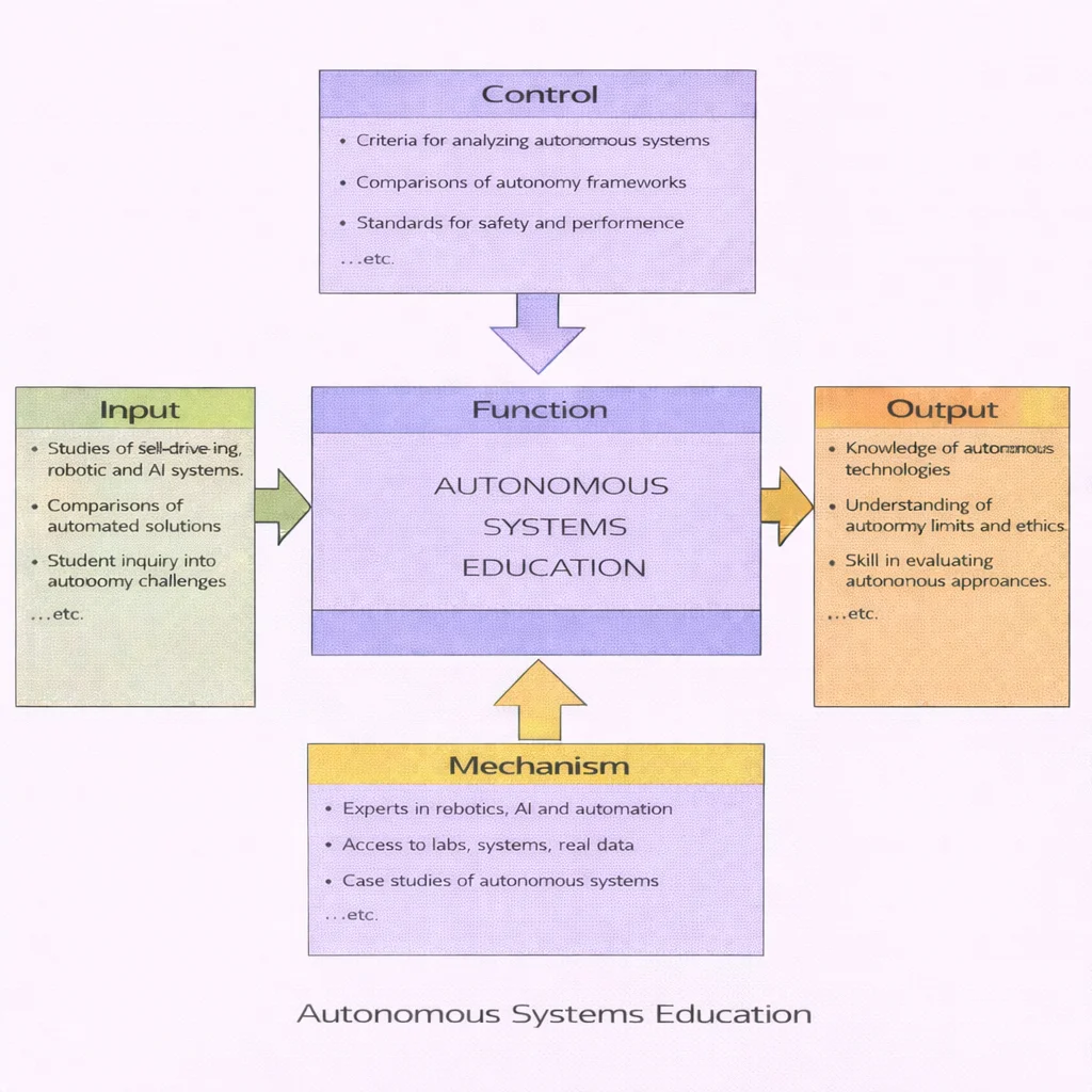
Autonomous Systems

Analysis: ACC maintains a longitudinal set-point speed or following distance using forward-facing radar. Full autonomy requires longitudinal and lateral control, 360-degree semantic segmentation, lane changes, interaction with traffic control devices, and predictive pedestrian behavior modeling.

Analysis: Downward-facing LiDAR/ultrasonic rangefinders for precision ground clearance, optical flow cameras for lateral drift tracking, an IMU to counteract wind gusts, and thermal cameras to verify the landing area is clear of humans and pets.

Analysis: High-frequency radio signals (such as GPS) attenuate rapidly in seawater. AUVs combine Doppler Velocity Logs (measuring speed relative to the seabed via acoustic Doppler shifts) with inertial navigation units (IMUs) and bathymetric sonar to maintain accurate position estimates over long dives.

Analysis: Distribution shifts occur when real-world sensory inputs differ significantly from training data distributions (such as unusual road work, novel vehicles, or rare weather). Neural networks can generate high-confidence incorrect predictions. Systems counter this with out-of-distribution detection, rule-based safety envelopes, and conservative fallback modes.

Analysis: Attack vectors include GPS spoofing, adversarial physical patches that fool camera vision models, and compromise of V2X communication links. Defenses require signed hardware roots of trust, encrypted CAN bus networks, and anomaly monitors checking for physically impossible vehicle states.

Scenario: An autonomous delivery drone navigates a straight flight corridor of total distance \(D = 500.0 \text{ m}\). Its nominal cruising speed is \(v_0 = 10.0 \text{ m}\cdot\text{s}^{-1}\). For \(50.0\%\) of the path, a strong localized headwind reduces its ground speed by \(20.0\%\). Determine the total transit time.

Step-by-Step Derivation:

$$ \begin{aligned} d_1 = d_2 &= \frac{500.0 \text{ m}}{2} = 250.0 \text{ m} \\ v_{\text{wind}} &= v_0 \times (1 - 0.20) = 10.0 \times 0.80 = 8.0 \text{ m}\cdot\text{s}^{-1} \\ t_1 &= \frac{d_1}{v_0} = \frac{250.0 \text{ m}}{10.0 \text{ m}\cdot\text{s}^{-1}} = 25.0 \text{ s} \\ t_2 &= \frac{d_2}{v_{\text{wind}}} = \frac{250.0 \text{ m}}{8.0 \text{ m}\cdot\text{s}^{-1}} = 31.25 \text{ s} \\ t_{\text{total}} &= t_1 + t_2 = 25.0 \text{ s} + 31.25 \text{ s} = 56.25 \text{ s} \end{aligned} $$

Answer & Conclusion: The drone completes the route in exactly \(56.25 \text{ seconds}\).

Scenario: A warehouse AMR samples its distance sensors every \(\Delta t = 0.50 \text{ s}\). If the robot completes \(N = 240\) discrete sampling steps while navigating an aisle, calculate the total traversal time in seconds and minutes.

Step-by-Step Derivation:

$$ \begin{aligned} T &= N \times \Delta t = 240 \times 0.50 \text{ s} = 120.0 \text{ s} \\ T_{\text{min}} &= \frac{120.0 \text{ s}}{60 \text{ s/min}} = 2.0 \text{ minutes} \end{aligned} $$

Answer & Conclusion: Total mission duration equals \(120.0 \text{ seconds}\) (or \(2.0 \text{ minutes}\)).

Scenario: An optical sensor system classifies \(1{,}000\) track objects with a baseline accuracy of \(98.0\%\). An algorithmic update increases accuracy by \(1.5\%\) absolute. Calculate the number of correct classifications before and after the update.

Step-by-Step Derivation:

$$ \begin{aligned} C_{\text{initial}} &= 1{,}000 \times 0.980 = 980 \text{ correct readings} \\ A_{\text{new}} &= 98.0\% + 1.5\% = 99.5\% \\ C_{\text{updated}} &= 1{,}000 \times 0.995 = 995 \text{ correct readings} \end{aligned} $$

Answer & Conclusion: Correct classifications increase from 980 to 995, reducing incorrect readings from 20 to 5.

Scenario: An autonomous shuttle travels \(D = 80.0 \text{ km}\) with an initial baseline travel time of \(t_0 = 1.50 \text{ hours}\). Heavy traffic reduces average speed by \(30.0\%\). Determine the new travel time in hours and minutes.

Step-by-Step Derivation:

$$ \begin{aligned} v_0 &= \frac{D}{t_0} = \frac{80.0 \text{ km}}{1.50 \text{ h}} \approx 53.33 \text{ km}\cdot\text{h}^{-1} \\ v_{\text{traffic}} &= v_0 \times (1 - 0.30) = 53.33 \times 0.70 \approx 37.33 \text{ km}\cdot\text{h}^{-1} \\ t_{\text{new}} &= \frac{D}{v_{\text{traffic}}} = \frac{80.0 \text{ km}}{37.33 \text{ km}\cdot\text{h}^{-1}} \approx 2.143 \text{ hours} \\ \text{Minutes} &= 0.143 \times 60 \approx 8.57 \text{ min} \approx 8 \text{ min } 34 \text{ s} \end{aligned} $$

Answer & Conclusion: Travel time increases to approximately \(2.14 \text{ hours}\) (or 2 hours, 8 minutes, and 34 seconds).

Scenario: A mobile surveillance robot runs for \(t_{\text{load}} = 4.0 \text{ hours}\) under full computational load. Engaging an edge power-optimization mode cuts compute draw by \(15.0\%\) and extends operating lifespan by \(25.0\%\). Calculate the new operating duration and the remaining compute profile.

Step-by-Step Derivation:

$$ \begin{aligned} t_{\text{extended}} &= 4.0 \text{ h} \times (1 + 0.25) = 4.0 \times 1.25 = 5.0 \text{ hours} \\ P_{\text{compute}} &= 100\% - 15.0\% = 85.0\% \end{aligned} $$

Answer & Conclusion: Battery life extends to \(5.0 \text{ hours}\) while maintaining \(85.0\%\) of maximum compute capacity.

Scenario: A municipal fleet of \(N = 50\) autonomous delivery robots averages \(d_0 = 12.0 \text{ km}\cdot\text{day}^{-1}\) per unit. Graph-theoretic route optimization shortens daily routes by \(10.0\%\). Determine the new single-robot distance and total fleet distance per day.

Step-by-Step Derivation:

$$ \begin{aligned} d_{\text{robot}} &= 12.0 \text{ km} \times (1 - 0.10) = 12.0 \times 0.90 = 10.8 \text{ km}\cdot\text{day}^{-1} \\ D_{\text{fleet}} &= 50 \times 10.8 \text{ km} = 540.0 \text{ km}\cdot\text{day}^{-1} \end{aligned} $$

Answer & Conclusion: Each robot travels \(10.8 \text{ km}\), reducing total daily fleet travel to \(540.0 \text{ km}\).

Scenario: An obstacle-avoidance algorithm achieves a \(95.0\%\) success rate across \(N = 80\) challenging maneuvers. A software update increases the success rate by \(3.0\%\) absolute. Calculate successful maneuvers before and after the update.

Step-by-Step Derivation:

$$ \begin{aligned} S_1 &= 80 \times 0.95 = 76 \text{ successful maneuvers} \\ R_2 &= 95.0\% + 3.0\% = 98.0\% \\ S_2 &= 80 \times 0.98 = 78.4 \rightarrow 78 \text{ fully completed maneuvers} \end{aligned} $$

Answer & Conclusion: Successful maneuvers increase from 76 to 78 (or \(78.4\) expected successes).

Scenario: A drone vision camera with native resolution of \(12.0 \text{ MP}\) implements a super-resolution model that increases effective pixel clarity by \(20.0\%\). Calculate the new effective resolution and the net pixel gain.

Step-by-Step Derivation:

$$ \begin{aligned} P_{\text{new}} &= 12.0 \text{ MP} \times (1 + 0.20) = 12.0 \times 1.20 = 14.4 \text{ MP} \\ \Delta P &= 14.4 \text{ MP} - 12.0 \text{ MP} = 2.4 \text{ MP} \end{aligned} $$

Answer & Conclusion: Effective resolution increases to \(14.4 \text{ MP}\), a net gain of \(2.4 \text{ MP}\).

Scenario: An industrial robotic workcell processes \(300 \text{ units/h}\). During an 8.0-hour shift, maintenance recalibration reduces throughput by \(12.0\%\) for \(30.0 \text{ minutes}\) every \(4.0 \text{ hours}\) (total maintenance: \(1.0 \text{ hour}\)). Calculate total units assembled during the shift.

Step-by-Step Derivation:

$$ \begin{aligned} t_{\text{normal}} &= 8.0 \text{ h} - 1.0 \text{ h} = 7.0 \text{ h} \\ t_{\text{maint}} &= 1.0 \text{ h} \\ R_{\text{maint}} &= 300 \text{ units/h} \times (1 - 0.12) = 300 \times 0.88 = 264 \text{ units/h} \\ U_{\text{normal}} &= 7.0 \text{ h} \times 300 \text{ units/h} = 2{,}100 \text{ units} \\ U_{\text{maint}} &= 1.0 \text{ h} \times 264 \text{ units/h} = 264 \text{ units} \\ U_{\text{total}} &= 2{,}100 + 264 = 2{,}364 \text{ units} \end{aligned} $$

Answer & Conclusion: The workcell produces \(2{,}364 \text{ units}\) across the shift.

Scenario: A vehicle LiDAR unit operates at a scan rate of \(f = 15.0 \text{ Hz}\) (\(15 \text{ scans/s}\)). The autonomous test car travels \(D = 2.0 \text{ km}\) (\(2{,}000.0 \text{ m}\)) at a constant speed of \(v = 20.0 \text{ m}\cdot\text{s}^{-1}\). Calculate total completed scans.

Step-by-Step Derivation:

$$ \begin{aligned} t_{\text{travel}} &= \frac{D}{v} = \frac{2{,}000.0 \text{ m}}{20.0 \text{ m}\cdot\text{s}^{-1}} = 100.0 \text{ s} \\ N_{\text{scans}} &= t_{\text{travel}} \times f = 100.0 \text{ s} \times 15.0 \text{ scans}\cdot\text{s}^{-1} = 1{,}500 \text{ scans} \end{aligned} $$

Answer & Conclusion: The LiDAR system completes \(1{,}500 \text{ complete scans}\) over the distance.

Scenario: An Autonomous Underwater Vehicle (AUV) records sonar data at \(R_0 = 5.0 \text{ MB}\cdot\text{min}^{-1}\) during a \(60.0\text{-minute}\) dive. An updated acoustic array increases data throughput by \(40.0\%\) and extends dive time to \(80.0 \text{ minutes}\). Compare total data gathered.

Step-by-Step Derivation:

$$ \begin{aligned} \text{Data}_{\text{orig}} &= 5.0 \text{ MB/min} \times 60.0 \text{ min} = 300.0 \text{ MB} \\ R_{\text{new}} &= 5.0 \text{ MB/min} \times (1 + 0.40) = 5.0 \times 1.40 = 7.0 \text{ MB/min} \\ \text{Data}_{\text{new}} &= 7.0 \text{ MB/min} \times 80.0 \text{ min} = 560.0 \text{ MB} \\ \Delta \text{Data} &= 560.0 \text{ MB} - 300.0 \text{ MB} = 260.0 \text{ MB} \end{aligned} $$

Answer & Conclusion: Total data increases from \(300.0 \text{ MB}\) to \(560.0 \text{ MB}\), an increase of \(86.7\%\).

Scenario: An ultrasonic proximity sensor has an initial false-positive error rate of \(8.0\%\). A hardware recalibration reduces the error rate by \(25.0\%\) relative. For \(2{,}000\) sample readings, calculate total errors before and after calibration.

Step-by-Step Derivation:

$$ \begin{aligned} E_{\text{initial}} &= 2{,}000 \times 0.080 = 160 \text{ errors} \\ \text{Rate}_{\text{new}} &= 8.0\% \times (1 - 0.25) = 8.0\% \times 0.75 = 6.0\% \\ E_{\text{updated}} &= 2{,}000 \times 0.060 = 120 \text{ errors} \\ \Delta E &= 160 - 120 = 40 \text{ fewer errors} \end{aligned} $$

Answer & Conclusion: False readings decrease from 160 down to 120, eliminating 40 false triggers.