Fluid Mechanics and Hydraulics: Flow, Pressure and Applications

Target Level: Undergraduate Engineering / Adv STEM

Estimated Study Time: 75–85 Minutes

Curricular Framework: Washington Accord / EUR-ACE

Principal Editor: Dr. Jacob Gan, PhD (Mich)

Fluid mechanics and hydraulics constitute the continuum physical science governing the statics, kinematics, and dynamics of liquids and gases. From laminar viscous transport and chaotic turbulent boundary layers to high-pressure electro-hydraulic circuits and turbomachinery, this discipline provides the mathematical foundation for converting fluid energy into controlled mechanical work.

Executive Curricular Takeaways:

Continuum Dynamics & Governing Equations: Formulate differential continuity, Navier-Stokes momentum equations, and the extended Bernoulli mechanical energy balance with major and minor friction losses.
Internal Pipe Networks & Boundary Layers: Evaluate the Colebrook-White implicit friction factor, Moody diagram regimes, boundary layer separation, and transient water hammer pressure wave acoustics.
Hydraulic Machinery & System Matching: Calculate pump total dynamic head (TDH), specific speed, Net Positive Suction Head (NPSH), cavitation inception margins, and open-channel gravity flows using Manning's formulation.

IDEF0 diagram of Fluid Mechanics and Hydraulics Education showing fluid properties and flow equations as inputs, guided by curriculum topics and evaluation metrics, enabled by test equipment and modeling software, producing prepared engineers and effective fluid systems.

Figure 1.0: IDEF0 Functional Architecture of Fluid Mechanics and Hydraulics Education (PREP4UNI.ONLINE Curricular Blueprint).

IDEF0 (Input-Control-Output-Mechanism) Systems Decomposition:

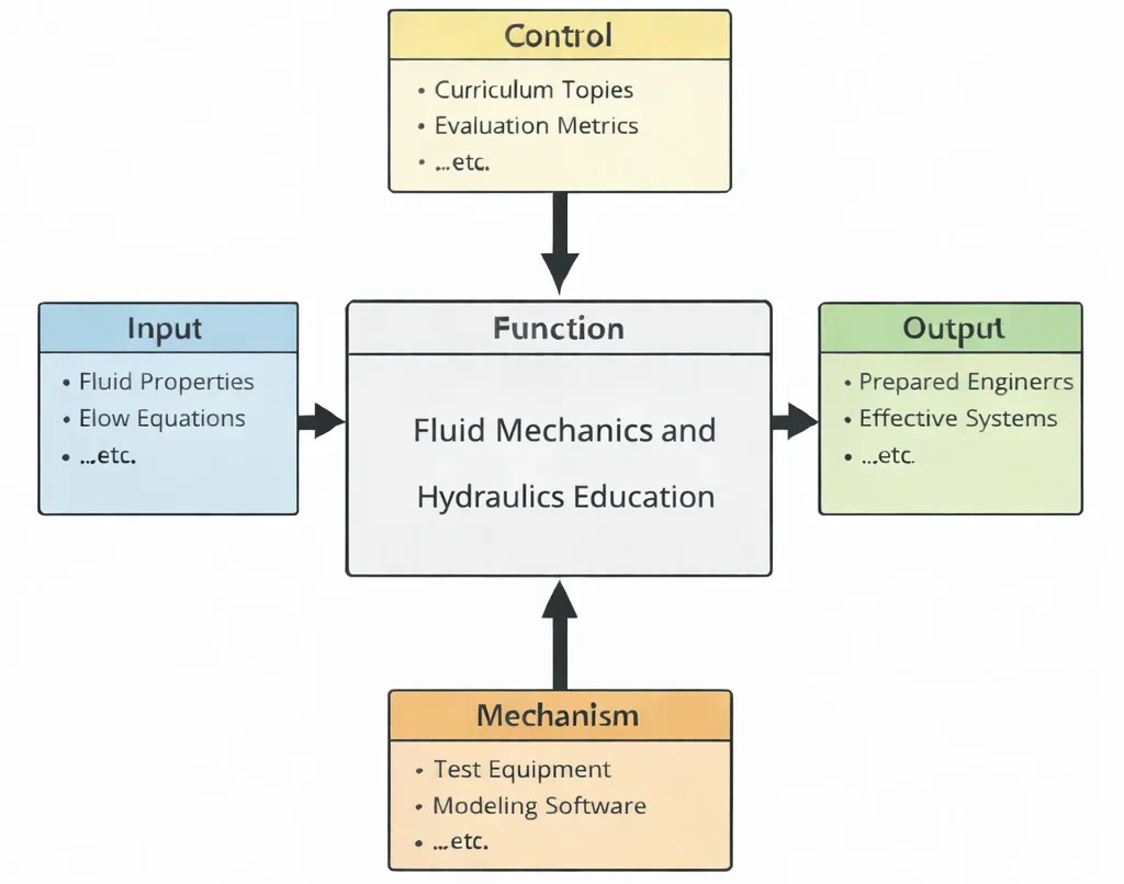
Inputs (Left): Thermophysical fluid properties (density ρ, dynamic viscosity μ, bulk modulus K), flow boundary conditions, pipeline geometry profiles, reservoir elevations, and fluid power duty cycles.
Controls (Top): Washington Accord/EUR-ACE engineering criteria, ASME B31.3 piping codes, ISO 4413 hydraulic fluid power standards, ANSI/HI pump test standards, and environmental discharge regulations.
Mechanisms (Bottom): Particle Image Velocimetry (PIV) flow rigs, high-pressure hydraulic testbenches, industrial pressure transducers, OpenFOAM/ANSYS Fluent CFD solvers, and SCADA-linked flow instrumentation.
Outputs (Right): Validated piping distribution networks, certified cavitation-free pumping plants, optimized aerodynamic/hydrodynamic profiles, and industry-ready fluid power engineers.

Mechanical & Thermal-Fluid Engineering Curriculum Cluster

Select any foundational pillar below to explore related modules across the PREP4UNI.ONLINE Mechanical Engineering series:

Mechanical Engineering (Hub)

Curricular synthesis, continuum mechanics foundation, cross-disciplinary trade-offs, and simulation testbeds.

Fluid Mechanics & Hydraulics

Navier-Stokes equations, Reynolds transport theorem, boundary layers, pipe friction, and hydraulic turbomachinery.

(Current Topic)

Thermodynamics & Heat Transfer

First and Second Laws, Rankine/Brayton/Carnot cycles, Fourier conduction, and multi-mode heat exchangers.

Solid Mechanics

Elasticity tensors, Mohr's circle, plane stress/strain, von Mises yield criteria, and beam bending formulations.

Mechanical Design & CAD

Parametric 3D solid modeling, GD&T (ASME Y14.5), fatigue failure theories (Goodman/Soderberg), and DFMA.

Control Systems

Laplace-domain transfer functions, root locus, Bode frequency response, state-space representations, and PID tuning.

Automotive Engineering

EV skateboard chassis, longitudinal/lateral vehicle dynamics, battery pack thermal runaway, and regenerative braking.

Manufacturing & Production

Subtractive machining dynamics, tool-wear equations, metal casting, polymer injection, and Industry 4.0 systems.

Robotics & Automation

Forward/inverse kinematics (Denavit-Hartenberg parameters), Jacobian dynamics, actuator sizing, and PLC architectures.

Biomechanical Engineering

Viscoelastic tissue mechanics, orthopaedic implant design, cardiovascular fluid-structure interaction, and biomaterials.

Vibrations & Acoustics

Lumped-parameter SDOF/MDOF systems, resonance, modal analysis, damping ratios, and acoustic wave equations.

Nanotechnology & Materials

Carbon nanotubes, graphene nanocomposites, grain boundary engineering (Hall-Petch), and surface functionalization.

Fluid Mechanics and Hydraulics research laboratory with flow visualization water tunnels, high-pressure actuators, and CFD monitors.

Figure 2.0: Cyber-physical fluid power laboratory: convergence of real-time particle imaging, high-pressure servo-hydraulics, and computational fluid dynamics.

Deep Technical Foundations: Analytical Formulations in Fluid Mechanics

Unlike rigid-body mechanics, fluids deform continuously under the application of shear stress. Analytical treatment requires formulating balance equations across infinitesimal control volumes, accounting for viscosity, convective acceleration, and frictional energy dissipation.

1. Incompressible Navier-Stokes Equations & Reynolds Transport

For an incompressible Newtonian fluid with constant density ρ and dynamic viscosity μ, the conservation of mass (continuity) and conservation of linear momentum in vector notation are expressed as:

$$\nabla \cdot \mathbf{v} = 0$$ $$\rho \left( \frac{\partial \mathbf{v}}{\partial t} + (\mathbf{v} \cdot \nabla)\mathbf{v} \right) = -\nabla P + \mu \nabla^2 \mathbf{v} + \rho \mathbf{g}$$

where v is the velocity vector field, P is static pressure, and g is gravitational body force. The non-linear advective acceleration term (v · ∇)v is responsible for vortex generation, flow separation, and the transition from laminar to turbulent regimes.

2. Extended Energy Equation & Pipe Network Head Loss

Applying the Reynolds Transport Theorem between two cross-sections (1 and 2) of a pipe network yields the extended mechanical energy balance expressed in head units (meters of fluid):

$$\frac{P_1}{\gamma} + \alpha_1 \frac{v_1^2}{2g} + z_1 + h_{\text{pump}} = \frac{P_2}{\gamma} + \alpha_2 \frac{v_2^2}{2g} + z_2 + h_{\text{turbine}} + h_L$$

where γ = ρg is specific weight, z is elevation head, and α is the kinetic energy correction factor (α = 2 for fully developed laminar flow; α ≈ 1.05 for turbulent flow). Total head loss h_L consists of major frictional losses h_f and minor fitting losses h_m:

$$h_f = f \left( \frac{L}{D} \right) \frac{v^2}{2g}, \qquad h_m = \sum K_L \frac{v^2}{2g}$$

where f is the Darcy-Weisbach friction factor. For laminar flow (Re < 2300), f = 64/Re. For turbulent flow (Re ≥ 4000), f is evaluated implicitly via the Colebrook-White equation or approximated explicitly by the Haaland equation:

$$\frac{1}{\sqrt{f}} \approx -1.8 \log_{10} \left[ \left( \frac{\varepsilon / D}{3.7} \right)^{1.11} + \frac{6.9}{\text{Re}} \right]$$

3. Centrifugal Turbomachinery, Affinity Laws & Cavitation Margins

Centrifugal pump performance scales with rotational speed N and impeller diameter D according to the homologous Affinity Laws:

$$\frac{Q_1}{Q_2} = \left(\frac{N_1}{N_2}\right)\left(\frac{D_1}{D_2}\right)^3, \qquad \frac{H_1}{H_2} = \left(\frac{N_1}{N_2}\right)^2\left(\frac{D_1}{D_2}\right)^2, \qquad \frac{P_{w,1}}{P_{w,2}} = \left(\frac{N_1}{N_2}\right)^3\left(\frac{D_1}{D_2}\right)^5$$

To prevent destructive bubble collapse (cavitation inception), the Net Positive Suction Head Available (NPSHA) at the pump suction nozzle must exceed the manufacturer's required Net Positive Suction Head (NPSHR) by an engineering safety margin:

$$\text{NPSHA} = \frac{P_{\text{atm}} - P_{\text{vapor}}}{\rho g} + z_{\text{suction}} - h_{L,\text{suction}} \ge \text{NPSHR} + \text{Margin}$$

Contemporary Computational Paradigms in Fluid Engineering

Industrial fluid systems development has evolved from purely empirical friction charts to accelerated multi-scale numerical modeling and cyber-physical infrastructure:

PINNs for Turbulent Boundary Layer Modeling

Physics-Informed Neural Networks incorporate the Reynolds-Averaged Navier-Stokes (RANS) momentum equations and Boussinesq turbulent eddy viscosity closures directly into the loss function. This allows rapid reconstruction of near-wall velocity profiles and shear stresses from sparse pressure tap arrays.

Fourier Neural Operators (FNOs) in Aerodynamics

Fourier Neural Operators learn infinite-dimensional continuum mappings from arbitrary 3D surface mesh geometry to external pressure and velocity fields. FNOs resolve full vehicle and turbine wake dynamics up to 1000 times faster than traditional Navier-Stokes mesh solvers.

Digital Twins of Municipal Water Networks

Cloud-coupled hydraulic digital twins solve real-time mass and momentum equations across thousands of pipe nodes using live SCADA flow and pressure telemetry. Utilizing Extended Kalman Filtering, the digital twin detects hidden subsurface main leaks and optimizes pump scheduling to reduce electrical grid demand.

Systems Engineering Trade-off Matrix

Designing fluid systems requires balancing pipe diameter, pump capital expenditure, frictional operating costs, transient pressure ratings, and cavitation limits:

Hydraulic Design Strategy	Primary Engineering Advantage	Bottlenecks & Failure Modes	Mitigation & Control Strategy
Small Pipe Diameter Selection (D ≪ D_opt)	Substantially reduces upfront piping material, valve procurement costs, structural trenching, and installation footprint.	Flow velocity scales inversely with area (v ∝ 1/D²), driving frictional head loss cubically (h_f ∝ 1/D⁵); escalates pump operating power and risk of erosion.	Perform life-cycle cost optimization balancing capital cost with annualized kilowatt-hour pumping costs over a 20-year service life.
High-Speed Centrifugal Pump Selection	Higher operational RPM yields compact casing dimensions, reduced impeller weight, and smaller electric motor frame sizes.	Significantly increases required Net Positive Suction Head (NPSHR ∝ N²); high risk of destructive vapor bubble collapse and impeller pitting.	Install inducer impellers ahead of main suction eye; elevate supply suction reservoir; lower operating fluid temperature to depress vapor pressure.
Fast-Closing Quarter-Turn Solenoid Valves	Enables near-instantaneous flow shutoff (< 0.1 s); prevents tank overfills; provides rapid emergency system isolation.	Rapid velocity destruction (Δv) generates severe acoustic pressure surge waves (Water Hammer), rupturing pipe joints and damaging instruments.	Install gas-charged bladder accumulators, surge anticipation relief valves, and program dual-speed slow-closing valve actuators.
High-Pressure Hydraulic Power (350+ bar)	Enables high actuator force density (F = P · A), allowing small cylinder diameters and compact, lightweight mobile equipment.	Elevated fluid bulk modulus loss from entrained air; extreme seal leakage; accelerated valve spool erosion and catastrophic pinhole injection hazards.	Specify multi-stage zero-clearance seals, micro-filtered synthetic esters or anti-wear mineral oils, and mandate high-strength seamless steel tubing.

Cross-Sector Industrial Case Studies

Heavy Mobile Earthmoving Equipment

Excavator hydraulic circuits deploy load-sensing axial piston pumps operating at 380 bar. Proportional closed-center directional valves modulate pilot fluid pressure, coordinating boom lifting and bucket curling while throttling flow to prevent pressure relief valve dumping.

Hydroelectric Pumped-Storage Generation

Francis pump-turbines operating under 450 meters of gross head convert mechanical potential energy into 300 MW of electrical power. Spiral casing geometries and draft tubes are shaped using CFD to maximize recovery of residual kinetic energy while preventing vortex core draft tube surging.

Transcontinental Hydrocarbon Pipelines

Multi-thousand-kilometer crude oil pipelines utilize series-staged multi-stage centrifugal booster pumps. Heavy crude viscosity is conditioned using polymeric drag-reducing agents (DRAs) injected at parts-per-million levels to suppress turbulent core eddies and reduce frictional pressure loss.

Semiconductor Chemical Delivery Systems

High-purity chemical etching tools utilize non-metallic PTFE bellows pumps and electro-pneumatic pinch valves to transport hydrofluoric acid at micro-flow rates under laminar conditions, eliminating metallic contamination and minimizing shear-induced micro-bubble formation.

Interactive Simulation: Venturi Tube Flow Dynamics & Bernoulli Solver

Evaluate real-time flow acceleration, dynamic pressure head conversion, static pressure drop (ΔP), and cavitation susceptibility across a variable-geometry Venturi pipeline constriction using our verified zero-crash canvas architecture.

Venturi Flow Dynamics & Bernoulli Simulator

STATUS: ACTIVE SOLVER

Inlet Velocity (v₁): 2.0 m/s

Throat Ratio (d₂/d₁): 0.50

Working Fluid:

Inlet Diameter (d₁): 0.20 m (Fixed)

Baseline Inlet Area A₁ = 0.0314 m²

Throat Velocity (v₂)

8.00 m/s

Pressure Drop (ΔP)

30.00 kPa

Volumetric Flow (Q)

0.063 m³/s

Kinetic Energy Head

3.26 m

Hydraulic Grade Line (Static Pressure) Streamline Velocity Profile Throat Constriction Minimum

Frequently Asked Questions: Fluid Mechanics & Hydraulic Systems

1. What distinguishes fluid mechanics from classical solid mechanics?

Solid mechanics evaluates materials that sustain static shear stress through finite elastic or plastic deformation strain (σ = Eε). A fluid is defined as a continuum substance that deforms continuously under the application of any non-zero shear stress, no matter how small (τ = μ du/dy). Consequently, fluid mechanics focuses on rates of deformation, velocities, and pressure fields rather than static equilibrium displacements.

2. Why does the Darcy-Weisbach equation supersede the empirical Hazen-Williams formula in modern engineering?

The Hazen-Williams formula is strictly empirical, valid only for water flowing at ordinary ambient temperatures within turbulent smooth-to-moderate pipes. In contrast, the Darcy-Weisbach equation is dimensionally homogeneous and universally applicable to any Newtonian fluid (liquid, gas, cryogen, oil) across laminar, transitional, and fully rough turbulent flow regimes, accurately accounting for viscosity and relative pipe roughness.

3. What physical conditions trigger cavitation inside hydraulic pumps and control valves?

Cavitation occurs whenever localized static fluid pressure drops below the saturation vapor pressure of the liquid at operating temperature (P < P_vapor). Liquid flash-boils into microscopic vapor cavities. When these bubbles travel into downstream regions of higher static pressure, they violently collapse within nanoseconds, producing localized micro-jets with impact pressures exceeding 1000 MPa, pitting metal impellers and causing severe structural vibration.

4. What is the fundamental physical difference between laminar and turbulent flow?

Laminar flow (Re < 2300 in circular conduits) is characterized by smooth, deterministic fluid layers sliding past one another with purely viscous momentum exchange. Turbulent flow (Re ≥ 4000) is governed by non-linear inertial advection, exhibiting three-dimensional chaotic fluctuations, swirling eddies, and intense momentum mixing. This mixing produces a blunt velocity profile and dramatically elevates wall shear stress and frictional pressure loss.

5. How does the hydraulic grade line (HGL) differ from the energy grade line (EGL)?

The Energy Grade Line (EGL) represents total mechanical energy head: $$\text{EGL} = \frac{P}{\gamma} + \frac{v^2}{2g} + z$$ The Hydraulic Grade Line (HGL) represents piezometric head (static pressure head plus elevation): $$\text{HGL} = \frac{P}{\gamma} + z$$ The vertical distance between the EGL and HGL is equal to the dynamic velocity head (v² / 2g). Whenever the physical pipe centerline rises above the HGL, static pressure in the pipe drops below atmospheric pressure, creating a vacuum siphon and risk of outgassing.

6. What causes water hammer, and how is the surge pressure wave velocity formulated?

Water hammer is an acoustic shock wave generated when fluid velocity is arrested rapidly (e.g., rapid valve closure). According to the Joukowsky equation, the peak surge pressure rise is ΔP = ρ · a · Δv, where a is the acoustic pressure wave propagation speed through the fluid-elastic pipe conduit: $$a = \sqrt{\frac{K / \rho}{1 + (K / E)(D / t)}}$$ where K is fluid bulk modulus, E is pipe Young's modulus, D is diameter, and t is wall thickness.

7. Why does Manning's equation apply strictly to open channel gravity flows?

Open channel flows possess a free liquid surface exposed directly to atmospheric pressure, meaning flow is driven entirely by the component of gravity acting along the channel bottom slope (S₀) rather than a closed-pipe pressure gradient. Manning's equation balances gravitational shear force against channel perimeter roughness resistance.

8. How does the Moody diagram classify the completely turbulent (rough pipe) regime?

At very high Reynolds numbers, the laminar viscous sublayer becomes thinner than the physical surface roughness projections (δ_sub < ε). The roughness elements protrude directly into the turbulent boundary layer, creating form drag. Viscosity drops out of the momentum balance, and the Darcy friction factor becomes completely independent of Reynolds number, depending solely on the relative roughness ratio (ε/D).

Student Practice & Accreditation Assessment Modules

Section 1: Interactive Knowledge Self-Assessment

Q1: Formulate the physical significance of the Reynolds number as a ratio of dynamic forces.

The Reynolds number is defined dimensionally as: $$\text{Re} = \frac{\rho v D}{\mu} = \frac{\rho v^2}{\mu (v / D)} \propto \frac{\text{Convective Inertial Forces}}{\text{Viscous Shear Forces}}$$ When Re ≪ 2300, viscous forces damp out perturbations, keeping streamlines laminar. When Re ≫ 4000, inertial forces overwhelm viscous damping, amplifying small velocity disturbances into self-sustaining turbulent eddies.

Q2: Differentiate between static pressure, dynamic pressure, and stagnation pressure in Bernoulli streamlines.

Static Pressure (P): The actual thermodynamic fluid pressure exerted on a surface moving parallel to the flow.
Dynamic Pressure (0.5ρv²): The kinetic energy per unit fluid volume representing pressure rise if fluid velocity were decelerated to zero isentropically.
Stagnation Pressure (P_stag): The total pressure measured at a zero-velocity stagnation point: $$P_{\text{stag}} = P + \frac{1}{2}\rho v^2$$

Q3: Why must pump operating points be located at the intersection of pump head and system head curves?

The pump head curve represents mechanical energy delivered by the impeller (H_p(Q) = H₀ − AQ²), while the system curve represents required static lift plus frictional and minor piping head loss (H_sys(Q) = Δz + BQ²). The physical operating point occurs uniquely where pump energy output exactly balances piping energy loss: $$H_p(Q^*) = H_{\text{sys}}(Q^*)$$

Q4: How does boundary layer separation induce aerodynamic form drag and hydraulic head loss?

When a fluid encounters an adverse pressure gradient (∂P / ∂x > 0) along a diverging surface, fluid particles in the near-wall viscous boundary layer lose kinetic energy. Eventually, wall shear stress reaches zero: $$\left. \frac{\partial u}{\partial y} \right|_{y=0} = 0$$ forcing the streamline flow to detach from the solid boundary. A turbulent low-pressure wake forms behind the body, creating substantial pressure imbalance and energy dissipation.

Q5: Why is Net Positive Suction Head Available (NPSHA) dependent on ambient barometric pressure and fluid temperature?

NPSHA measures suction head margin above fluid vapor pressure: $$\text{NPSHA} = \frac{P_{\text{atm}} - P_{\text{vapor}}(T)}{\rho g} + z_s - h_{L,s}$$ Atmospheric pressure provides the driving force pushing liquid into the pump suction eye. Higher fluid temperatures raise saturation vapor pressure exponentially via the Clausius-Clapeyron relation, drastically depressing NPSHA toward cavitation thresholds.

Q6: What causes hydraulic jump in open channel gravity flows, and what energy transformation occurs?

A hydraulic jump occurs when open channel flow transitions rapidly from high-velocity supercritical flow (Froude number Fr > 1) to low-velocity subcritical flow (Fr < 1). The jump manifests as an abrupt turbulent standing wave that dissipates large quantities of mechanical kinetic energy into turbulent thermal heat, protecting downstream channel beds from severe erosion.

Q7: Why do positive displacement pumps require pressure relief valves, while centrifugal pumps can be operated against closed valves?

Positive displacement pumps trap fixed fluid volumes per stroke or revolution. If the discharge line is deadheaded, fluid pressure rises toward infinity until motor stall or physical casing rupture occurs. Centrifugal pumps are dynamic machines whose maximum shutoff head is naturally capped by impeller tip speed (H₀ ≈ v_tip² / 2g), permitting short periods of closed-valve operation without immediate structural bursting.

Q8: Formulate how Pascal's Law enables force multiplication in closed hydraulic presses.

According to Pascal's Law, static pressure applied to an enclosed incompressible fluid is transmitted undiminished in all directions: $$P_1 = P_2 \Rightarrow \frac{F_1}{A_1} = \frac{F_2}{A_2} \Rightarrow F_2 = F_1 \left( \frac{A_2}{A_1} \right)$$ By sizing the output piston area A₂ much larger than input piston area A₁, input force is amplified by the exact geometric area ratio.

Section 2: Analytical & Scenario-Based Case Studies

Case Study 2.1: Severe Impeller Cavitation Pitting in a Boiler Feedwater Pumping Station POWER PLANT HYDRAULICS

Scenario: A 400-kW multi-stage centrifugal boiler feedwater pump suffered catastrophic impeller erosion, violent vibration (18 mm/s RMS), and loud crackling noise after boiler operating temperature was raised from 75°C to 95°C.

Engineering Evaluation:
1. Vapor Pressure Surge: Elevating water temperature to 95°C increased saturation vapor pressure from P_vapor(75°C) = 38.6 kPa to P_vapor(95°C) = 84.5 kPa.
2. NPSH Erosion: With atmospheric pressure P_atm = 101.3 kPa, suction head margin dropped: $$\text{NPSHA} = \frac{101.3 - 84.5}{9.81 \cdot 0.962} + 1.2 - 0.9 = 1.78 + 0.3 = 2.08 \text{ m}$$ Because pump required suction head was NPSHR = 3.60 m, the system operated in deep cavitation (NPSHA ≪ NPSHR). Vapor cavities collapsed on the low-pressure blade suction surfaces, eroding 4 mm of chrome-steel alloy.
Corrective Engineering Action: Elevate the deaerator storage tank by 3.5 meters to increase static suction head z_s, and install an axial booster inducer upstream of the first-stage impeller eye to lower NPSHR to 1.8 meters.

Case Study 2.2: Water Hammer Pipe Rupture Following Emergency Valve Closure TRANSIENT DYNAMICS

Scenario: A 600-mm diameter ductile iron cooling water supply main ruptured at an elbow fitting following a sudden 0.25-second emergency trip of an automated butterfly valve, flooding a municipal pumping station.

Engineering Evaluation:
The pipeline carried water at v₀ = 3.2 m/s over a length of L = 1200 m. Acoustic wave velocity was a = 1050 m/s. The critical pipeline closure time was: $$T_{\text{crit}} = \frac{2L}{a} = \frac{2 \cdot 1200}{1050} \approx 2.29 \text{ s}$$ Because valve closure time (t_c = 0.25 s) was much less than T_crit, rapid closure occurred. Applying the Joukowsky equation: $$\Delta P_{\text{surge}} = \rho \cdot a \cdot \Delta v = 1000 \cdot 1050 \cdot 3.2 = 3.36 \times 10^6 \text{ Pa} = 33.6 \text{ bar}$$ Adding steady operating pressure (6.0 bar), total internal pressure reached 39.6 bar, exceeding the pipeline's 16-bar maximum design rating and shearing fitting bolts.
Corrective Engineering Action: Retrofit the valve actuator with a two-stage hydraulic damper enforcing closure time t_c ≥ 8.0 s, and install a 15-m³ nitrogen-charged bladder surge accumulator upstream of the valve.

Case Study 2.3: Hydraulic Cylinder Stick-Slip Oscillation and Thermal Seal Breakdown SERVO-HYDRAULICS

Scenario: A 200-ton hydraulic forging press exhibited severe low-speed positioning chatter (stick-slip vibration at 3 Hz) and blackened, degraded polyurethane piston seals after 600 hours of continuous cycling.

Engineering Evaluation:
1. Viscosity Degradation: The hydraulic reservoir lacked adequate oil cooling; bulk oil temperature reached 88°C, reducing mineral oil kinematic viscosity from 46 cSt to 8.2 cSt.
2. Boundary Friction: Thin fluid film allowed metal-to-metal boundary contact between the piston head and cylinder wall. The static friction coefficient was substantially higher than kinetic friction (μ_s ≫ μ_k), creating non-linear stick-slip hunting during micro-feed motions.
Corrective Engineering Action: Install an air-blast oil-water heat exchanger maintaining bulk oil temperature between 45°C and 55°C, and replace standard polyurethane packings with low-friction bronze-filled PTFE (Teflon) step-seals incorporating elastomeric O-ring energizers.

Case Study 2.4: Severe Flow Separation and Draft Tube Surging in a Francis Hydro Turbine TURBOMACHINERY

Scenario: A 75-MW Francis hydro turbine operating at 45% partial load generated deep acoustic pressure pulsations (0.3 times shaft speed) that rattled the powerhouse foundation.

Engineering Evaluation:
Operating at partial load causes water exiting the runner blades to retain substantial residual swirl. In the diverging conical draft tube, this swirling flow encounters an adverse pressure gradient, producing an unstable precessing helical vortex core (the "draft tube rope"). Pressure fluctuations registered amplitudes of ±18% of total head, exciting powerhouse structural resonance.
Corrective Engineering Action: Inject compressed atmospheric air into the center of the draft tube below the runner cone to cushion vortex pulsations, and restrict continuous turbine operation to the high-efficiency operating zone (70–100% load).

Case Study 2.5: Severe Frictional Choking in a Compressed Natural Gas Pipeline COMPRESSIBLE FLOW

Scenario: A 15-kilometer gas transmission pipeline experienced sharp pressure drop and severe acoustic screaming when supplying an industrial combined-cycle power plant during winter peak demand.

Engineering Evaluation:
High volumetric mass flow rates accelerated compressible natural gas velocity to M = 0.45. In long pipelines, Fanno line flow mechanics dictate that wall friction accelerates subsonic compressible flow toward Mach 1: $$\frac{dM^2}{dx} = \frac{\gamma M^4 \left(1 + \frac{\gamma - 1}{2} M^2\right)}{1 - M^2} \left( \frac{4f}{D} \right) \gt 0$$ As velocity escalated near the downstream discharge header, frictional pressure drop increased exponentially, causing delivery pressure to drop below turbine inlet requirements.
Corrective Engineering Action: Loop the pipeline by installing an identical parallel 400-mm line over the final 8 kilometers, halving gas mass flux and restoring delivery pressure above 45 bar.

Case Study 2.6: Erosion Corrosion Failure in an HVAC Chilled Water Copper Header BUILDING SERVICES

Scenario: A commercial building chilled water system suffered multiple pinhole leaks and copper wall thinning along short-radius 90° elbow fittings after three years of operation.

Engineering Evaluation:
To minimize piping material costs, designers selected 50-mm copper headers delivering flow velocities v = 3.8 m/s. Standard ASHRAE codes recommend capping copper water velocities at 1.5–2.0 m/s. The high flow velocity and secondary Dean vortex turbulence at sharp bends stripped the protective copper oxide passivation film, causing continuous erosion-corrosion wear.
Corrective Engineering Action: Upsize distribution headers to 75-mm diameter, lowering velocity to 1.68 m/s, and specify long-radius smooth-sweep elbows (R/D ≥ 1.5).

Case Study 2.7: Bridge Scour Collapse During Storm Flood Waves CIVIL HYDRAULICS

Scenario: A multi-span highway bridge over a gravel river collapsed when floodwaters undermined the spread footing of its central pier during a 100-year storm event.

Engineering Evaluation:
Bridge piers obstruct open-channel flow, inducing a downward stagnation pressure gradient that drives a high-velocity horseshoe vortex at the pier base. Local bed shear stress exceeded critical sediment movement thresholds: $$\tau_{\text{bed}} \gg \tau_{\text{crit}}$$ The vortex excavated a 4.5-meter deep scour hole around the central pier footing, eroding bearing gravel and causing structural foundation tilting.
Corrective Engineering Action: Install deep-driven drilled shaft piles extending 12 meters into bedrock, and armor the riverbed surrounding the piers with engineered riprap boulders sized to resist peak flood shear forces.

Section 3: Step-by-Step Quantitative Worked Examples

Worked Example 3.1: Hydrostatic Pressure, Gage Head & Total Base Force FLUID STATICS

Problem Statement: A vertical cylindrical storage reservoir with flat base area A = 2.00 m² is filled with water of density ρ = 1000 kg/m³ to a free-surface height h = 5.00 m. Atmospheric pressure is P_atm = 101.325 kPa, and gravitational acceleration is g = 9.81 m/s². Calculate:
(a) The hydrostatic gauge pressure (P_gage) at the reservoir floor in kPa.
(b) The absolute pressure (P_abs) at the reservoir floor in kPa.
(c) The total downward resultant force (F_base) exerted by the fluid on the flat floor in kilonewtons.

Step 1: Compute Hydrostatic Gauge Pressure (P_gage) $$P_{\text{gage}} = \rho \cdot g \cdot h = (1000 \text{ kg/m}^3) \cdot (9.81 \text{ m/s}^2) \cdot (5.00 \text{ m}) = 49{,}050 \text{ Pa} = 49.05 \text{ kPa}$$

Step 2: Compute Absolute Pressure (P_abs) $$P_{\text{abs}} = P_{\text{gage}} + P_{\text{atm}} = 49.05 \text{ kPa} + 101.325 \text{ kPa} = 150.375 \text{ kPa}$$

Step 3: Compute Total Hydrostatic Downward Base Force (F_base) $$F_{\text{base}} = P_{\text{gage}} \cdot A = (49{,}050 \text{ N/m}^2) \cdot (2.00 \text{ m}^2) = 98{,}100 \text{ N} = 98.10 \text{ kN}$$

Engineering Interpretation: The 5-meter water column generates 49.05 kPa of gauge pressure, imposing a sustained 98.1 kN mechanical load on the tank floor. Sizing of anchor bolts and floor plate thicknesses must be engineered to resist this hydrostatic load while checking against soil settlement.

Worked Example 3.2: Continuity Balance and Velocity Acceleration Across a Pipe Reducer INTERNAL CONDUIT FLOW

Problem Statement: Water (ρ = 1000 kg/m³) flows through a horizontal pipeline that constricts from cross-sectional area A₁ = 0.080 m² to A₂ = 0.020 m². Velocity in the upstream pipe is v₁ = 2.00 m/s. Calculate:
(a) The total volumetric flow rate (Q) in m³/s and mass flow rate (ṁ) in kg/s.
(b) The flow velocity in the constricted section (v₂) in m/s.
(c) The change in kinetic energy velocity head (Δh_v) across the transition in meters of water.

Step 1: Compute Volumetric and Mass Flow Rate $$Q = A_1 \cdot v_1 = (0.080 \text{ m}^2) \cdot (2.00 \text{ m/s}) = 0.160 \text{ m}^3/\text{s}$$ $$\dot{m} = \rho \cdot Q = (1000 \text{ kg/m}^3) \cdot (0.160 \text{ m}^3/\text{s}) = 160.0 \text{ kg/s}$$

Step 2: Apply Continuity for Incompressible Flow (A₁v₁ = A₂v₂) $$v_2 = \frac{Q}{A_2} = \frac{0.160 \text{ m}^3/\text{s}}{0.020 \text{ m}^2} = 8.00 \text{ m/s}$$

Step 3: Compute Change in Kinetic Energy Velocity Head $$h_{v,1} = \frac{v_1^2}{2g} = \frac{(2.00)^2}{2 \cdot 9.81} = \frac{4.0}{19.62} \approx 0.2039 \text{ m}$$ $$h_{v,2} = \frac{v_2^2}{2g} = \frac{(8.00)^2}{2 \cdot 9.81} = \frac{64.0}{19.62} \approx 3.2620 \text{ m}$$ $$\Delta h_v = h_{v,2} - h_{v,1} = 3.2620 - 0.2039 = 3.0581 \text{ m}$$

Engineering Interpretation: Reducing the conduit area by a factor of 4 quadruples flow velocity from 2.0 m/s to 8.0 m/s. This elevates velocity head from 0.20 m to 3.26 m. According to Bernoulli principles, this acceleration converts static pressure head into dynamic head, creating an upstream-to-downstream pressure drop.

Worked Example 3.3: Reynolds Number & Flow Regime Transition Classification VISCOUS MOMENTUM DYNAMICS

Problem Statement: Water at 20°C (ρ = 998.2 kg/m³, dynamic viscosity μ = 1.002 × 10⁻³ Pa·s) flows through a smooth circular pipe of inner diameter D = 0.050 m (50 mm) at a mean velocity v = 1.20 m/s.
(a) Compute the Reynolds number (Re).
(b) Classify the flow regime (laminar, transitional, or turbulent).
(c) Determine the critical velocity (v_crit) below which flow is guaranteed to remain laminar (taking Re_crit = 2300).

Step 1: Compute Reynolds Number (Re) $$\text{Re} = \frac{\rho \cdot v \cdot D}{\mu} = \frac{(998.2 \text{ kg/m}^3) \cdot (1.20 \text{ m/s}) \cdot (0.050 \text{ m})}{1.002 \times 10^{-3} \text{ Pa}\cdot\text{s}} = \frac{59.892}{1.002 \times 10^{-3}} \approx 59{,}772$$

Step 2: Classify Flow Regime

Because Re ≈ 59,800 is significantly greater than 4000, the flow is fully established Turbulent Flow.

Step 3: Calculate Critical Laminar Velocity Threshold (v_crit) $$v_{\text{crit}} = \frac{\text{Re}_{\text{crit}} \cdot \mu}{\rho \cdot D} = \frac{(2300) \cdot (1.002 \times 10^{-3} \text{ Pa}\cdot\text{s})}{(998.2 \text{ kg/m}^3) \cdot (0.050 \text{ m})} = \frac{2.3046}{49.91} \approx 0.04618 \text{ m/s} = 4.62 \text{ cm/s}$$

Engineering Interpretation: Operating at 1.2 m/s produces an inertia-dominated turbulent regime (Re ≈ 59,800) with extensive mixing and high friction factor. Water flow in this 50-mm pipe remains laminar only at speeds below 4.6 cm/s, illustrating why commercial pipelines operate almost exclusively in the turbulent regime.

Worked Example 3.4: Pascal Hydraulic Jack Force Amplification & Stroke Sizing FLUID POWER TRANSMISSION

Problem Statement: A hydraulic workshop press utilizes a hand pump piston of radius r₁ = 0.020 m (20 mm) connected to an output ram cylinder of radius r₂ = 0.100 m (100 mm). The circuit is charged with ISO VG 46 mineral oil. A technician applies an input force F₁ = 500 N to the input piston. Calculate:
(a) The internal hydraulic line pressure (P_sys) in kPa and bar.
(b) The output lifting force (F₂) exerted by the large ram in kilonewtons.
(c) The ideal mechanical force multiplication advantage (MA).
(d) The stroke displacement of the load ram (s₂) if the hand pump piston travels s₁ = 0.050 m (50 mm).

Step 1: Compute Cross-Sectional Areas and Hydraulic Pressure $$A_1 = \pi r_1^2 = \pi (0.020)^2 = 0.0004\pi \approx 1.2566 \times 10^{-3} \text{ m}^2$$ $$A_2 = \pi r_2^2 = \pi (0.100)^2 = 0.0100\pi \approx 3.1416 \times 10^{-2} \text{ m}^2$$ $$P_{\text{sys}} = \frac{F_1}{A_1} = \frac{500 \text{ N}}{1.2566 \times 10^{-3} \text{ m}^2} \approx 397{,}887 \text{ Pa} = 397.89 \text{ kPa} \approx 3.98 \text{ bar}$$

Step 2: Compute Output Lifting Force (F₂ = P_sys · A₂) $$F_2 = F_1 \left( \frac{A_2}{A_1} \right) = 500 \text{ N} \cdot \left( \frac{r_2^2}{r_1^2} \right) = 500 \cdot \left(\frac{0.10}{0.02}\right)^2 = 500 \cdot (5)^2 = 500 \cdot 25 = 12{,}500 \text{ N} = 12.50 \text{ kN}$$

Step 3: Mechanical Advantage (MA) and Stroke Displacement (s₂) $$\text{MA} = \frac{F_2}{F_1} = 25.0$$ $$\text{Volume Conservation: } V_1 = V_2 \Rightarrow A_1 \cdot s_1 = A_2 \cdot s_2$$ $$s_2 = s_1 \left( \frac{A_1}{A_2} \right) = \frac{0.050 \text{ m}}{25.0} = 0.0020 \text{ m} = 2.00 \text{ mm}$$

Engineering Interpretation: Pascal's principle delivers a 25-fold force amplification, converting 500 N into a 12.5 kN lifting force at an operating pressure of 3.98 bar. In accordance with work conservation, this force multiplication requires trading stroke distance: a 50-mm pump stroke moves the heavy load by 2.0 mm.

Worked Example 3.5: Darcy-Weisbach Pipeline Frictional Head Loss & Pumping Power PIPING NETWORK DESIGN

Problem Statement: A steel pipeline of length L = 100 m and inside diameter D = 0.100 m conveys hydraulic oil of density ρ = 870 kg/m³ at a mean flow velocity v = 3.00 m/s. The Darcy friction factor is f = 0.025. Gravity is g = 9.81 m/s². Calculate:
(a) The frictional head loss (h_f) in meters of fluid.
(b) The frictional pressure drop (ΔP_f) along the 100-meter pipe in kPa.
(c) The theoretical pumping power (P_pump) required solely to overcome this line friction in kilowatts.

Step 1: Compute Frictional Head Loss via Darcy-Weisbach $$h_f = f \left( \frac{L}{D} \right) \frac{v^2}{2g} = (0.025) \cdot \left( \frac{100 \text{ m}}{0.100 \text{ m}} \right) \cdot \frac{(3.00 \text{ m/s})^2}{2 \cdot 9.81 \text{ m/s}^2}$$ $$h_f = 0.025 \cdot 1000 \cdot \frac{9.00}{19.62} = 25.0 \cdot 0.458716 \approx 11.468 \text{ m}$$

Step 2: Compute Frictional Pressure Drop (ΔP_f) $$\Delta P_f = \rho \cdot g \cdot h_f = (870 \text{ kg/m}^3) \cdot (9.81 \text{ m/s}^2) \cdot (11.468 \text{ m}) = 8534.7 \cdot 11.468 \approx 97{,}876 \text{ Pa} \approx 97.88 \text{ kPa}$$

Step 3: Compute Volumetric Flow Rate and Pumping Power $$A = \frac{\pi}{4} D^2 = \frac{\pi}{4} (0.10)^2 \approx 7.854 \times 10^{-3} \text{ m}^2$$ $$Q = A \cdot v = (7.854 \times 10^{-3} \text{ m}^2) \cdot (3.00 \text{ m/s}) \approx 0.023562 \text{ m}^3/\text{s}$$ $$P_{\text{pump}} = \Delta P_f \cdot Q = (97{,}876 \text{ N/m}^2) \cdot (0.023562 \text{ m}^3/\text{s}) \approx 2306.2 \text{ W} \approx 2.31 \text{ kW}$$

Engineering Interpretation: Fluid friction dissipates 11.47 meters of head (97.9 kPa) over 100 meters, requiring 2.31 kW of continuous hydraulic shaft power. If pump-motor efficiency is η = 78%, electrical supply draw is 2.96 kW.

Worked Example 3.6: Open-Channel Normal Velocity & Discharge via Manning's Equation OPEN CHANNEL HYDRAULICS

Problem Statement: A rectangular finished concrete stormwater channel of width b = 2.50 m carries water at uniform normal depth y = 1.00 m. The bed slope is S₀ = 0.0010 (0.1% grade), and Manning's roughness coefficient is n = 0.015 s/m^1/3. Calculate:
(a) The flow area (A), wetted perimeter (P_w), and hydraulic radius (R_h).
(b) The mean cross-sectional flow velocity (v) in m/s using Manning's equation.
(c) The total volumetric discharge capacity (Q) in m³/s.
(d) The Froude number (Fr) and classify whether the flow is subcritical or supercritical.

Step 1: Compute Geometric Parameters (A, P_w, R_h) $$A = b \cdot y = (2.50 \text{ m}) \cdot (1.00 \text{ m}) = 2.50 \text{ m}^2$$ $$P_w = b + 2y = 2.50 + 2(1.00) = 4.50 \text{ m}$$ $$R_h = \frac{A}{P_w} = \frac{2.50 \text{ m}^2}{4.50 \text{ m}} \approx 0.5556 \text{ m}$$

Step 2: Evaluate Flow Velocity via Manning's Formulation $$v = \frac{1}{n} R_h^{2/3} S_0^{1/2} = \left(\frac{1}{0.015}\right) \cdot (0.5556)^{2/3} \cdot (0.0010)^{1/2}$$ $$(0.5556)^{0.6667} \approx 0.6757, \qquad \sqrt{0.0010} \approx 0.031623$$ $$v = 66.667 \cdot 0.6757 \cdot 0.031623 \approx 1.4245 \text{ m/s}$$

Step 3: Compute Total Volumetric Discharge (Q) $$Q = A \cdot v = (2.50 \text{ m}^2) \cdot (1.4245 \text{ m/s}) \approx 3.561 \text{ m}^3/\text{s}$$

Step 4: Compute Froude Number (Fr) and Classify Flow Regime $$D_h = \frac{A}{T_{\text{top}}} = \frac{2.50}{2.50} = 1.00 \text{ m}$$ $$\text{Fr} = \frac{v}{\sqrt{g D_h}} = \frac{1.4245 \text{ m/s}}{\sqrt{9.81 \cdot 1.00}} = \frac{1.4245}{3.1321} \approx 0.4548$$

Because Fr = 0.455 < 1.0, the flow is established Subcritical Flow (tranquil regime).

Engineering Interpretation: The concrete channel conveys 3.56 m³/s of stormwater at a velocity of 1.42 m/s. Because the Froude number is 0.455 (< 1), the flow is subcritical: gravity waves can propagate upstream, allowing downstream control structures (such as weirs and culverts) to govern water depth without triggering uncontrolled hydraulic jumps.

← Back to Mechanical Engineering Hub

Fluid Mechanics and Hydraulics