Prepare for University Studies & Career Advancement
AC Circuits and Impedance
AC circuits are circuits in which voltage and current change direction repeatedly with time. Unlike direct-current circuits, where current usually flows steadily in one direction, alternating-current circuits involve continuous variation. This makes AC behaviour richer: voltage, current, resistance, capacitance, inductance, frequency, and phase all become important parameters.
Impedance is the central concept that helps students master AC circuits. In DC networks, resistance describes how strongly a component opposes current. In AC environments, capacitors and inductors also oppose current, but their opposition depends directly on driving frequency and shifts the timing relationship between voltage and current. Impedance combines resistance and frequency-dependent effects into one unified network parameter.
This page completes the first Electrical Circuits pathway by moving from steady current to time-varying current. Students who understand impedance are better prepared for filtering networks, resonance tuning, signal processing, power grids, audio electronics, communication links, and advanced electromagnetic field theory.
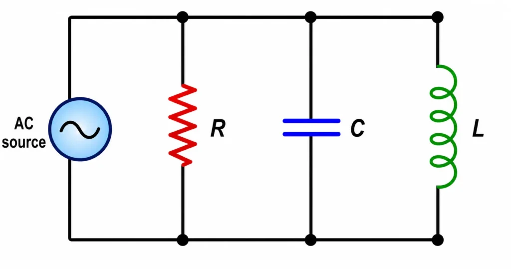
An AC circuit may contain resistance, capacitance, and inductance, each affecting alternating current in a different way.
This illustration shows an AC source connected to three important circuit components: a resistor, a capacitor, and an inductor. In an AC circuit, these components do not respond in the same way. The resistor opposes current directly, the capacitor stores and releases energy in an electric field, and the inductor stores and releases energy in a magnetic field. Together, they help students understand why AC circuits depend on impedance, reactance, frequency, and phase difference.
Electrical Circuits Learning Pathway
This page follows from Ohm’s law, series and parallel circuits, Kirchhoff’s laws, and RC circuits. It extends circuit thinking into alternating current, where frequency and phase become essential.
Connects resistance with capacitance to explain charging, discharging, exponential change, and time delay in circuits.
AC Circuits and Impedance
Details conservative forces, kinetic-to-potential transformations, and the energy baselines fueling system cycles.
2. The Core Intuition (Without Calculus)
Circuit behaviour depends strongly on how components react to changing currents. In the absence of steady state parameters, reactive components act entirely differently depending on driving frequencies.
Work/Energy Transfer: The process of moving electrical potential through reactive impedances into active thermal dissipation or storage matrices.
Energy States: Mechanical parameters map to electrostatics; where capacitors track electric potential energy fields and inductors handle magnetic field energy reserves.
Power Flow: Sinusoidal scaling means output delivery changes coordinates constantly based on phase parameter differences.
Quick Check: Energy Accounting & Intuition
Question 1: An ideal AC source drives an isolated capacitor node. Over a complete electrical period cycle, how much active power is permanently dissipated by the capacitor into thermal waste?
Conceptual Solution: Exactly zero Joules. An ideal capacitor charges during the first quarter-cycle, storing electrostatic potential, and returns all captured energy back to the source field during discharge steps. It generates reactive power opposition, but consumes zero active power.
Question 2: A load has a massive phase difference angle where current lags voltage by 90°. Is this circuit network delivering useful power to an active load?
Conceptual Solution: No, the real power output evaluates to zero. Using the expression \(P = VI \cos(\theta)\), where \(\theta = 90^\circ\), the term \(\cos(90^\circ) = 0\). This system is completely reactive, meaning energy cycles inside local fields without transferring out to do work.
2. Demystifying Phase and Sign Conventions
In alternating current regimes, parameters are time-dependent profiles. Signs and directions update continuously, meaning tracking phase vectors dominates over standard algebraic metrics.
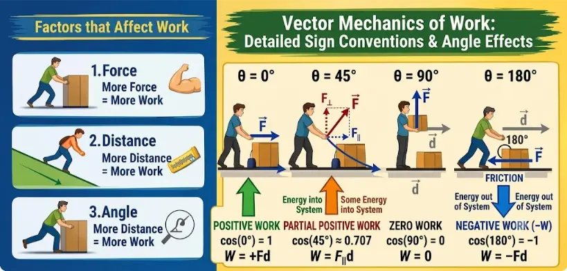
Complete Vector Mapping of Work Sign Conventions and Energy Transfer.
Quick Check: AC Parameter Sign Dynamics
Question 1: An ideal inductor is connected to a sinusoidal generator path. Does the resulting current wave lag or lead the driving potential drop vector?
Conceptual Solution: The current vector lags the voltage vector by exactly \(90^\circ\). Inductors inherently oppose immediate current updates, forcing the voltage profile to peak before the charge drift velocity can scale up.
3. The Calculus Bridge (University Level)
Steady-state models fail during high-speed transient windows. When analyzing capacitor elements, current tracks directly as the time derivative of electrical potential, forcing the network equations into differential formats:
$$
i(t) = C\frac{dV}{dt}
$$
Similarly, an inductor generates an electromotive force profile that tracks the instantaneous rate of current update:
$$
V(t) = L\frac{di}{dt}
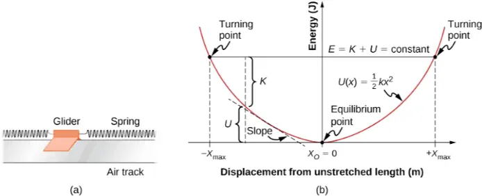
$$The geometric mapping of a conservative potential energy curve, showing how the slope links visually to restoring force behaviors.
Quick Check: Transitioning to University Calculus
Question 1: The time-varying voltage profile running across a \(2\text{ F}\) capacitor element is defined as \(V(t) = 4t^3\). Determine the expression for the current profile at time \(t = 2\text{ s}\).
Numerical Solution: Apply the time-derivative equation:
Heavy distribution sub-stations utilize alternating current step-up transformer topologies to step up potential line values, minimizing line-loss dissipation factors over geographical scales.
Automotive Regenerative Brakes
Rectification Profiles
Automotive hybrid rectifiers convert the time-varying sinusoidal currents captured from mechanical braking loops into uniform direct currents to charge DC storage cells.
Spacecraft Gravity Assists
Inductive Telemetry Isolation
Deep-space hardware channels high-frequency radio frequency paths using isolated inductive links to ensure vital logic computing cores are protected against cosmic plasma static.
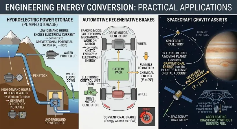
Systems diagram of diverse real-world engineering applications of energy conversion, highlighting efficiency strategies in hydroelectric storage, electric vehicles, and deep space navigation.
5. Common Misconceptions
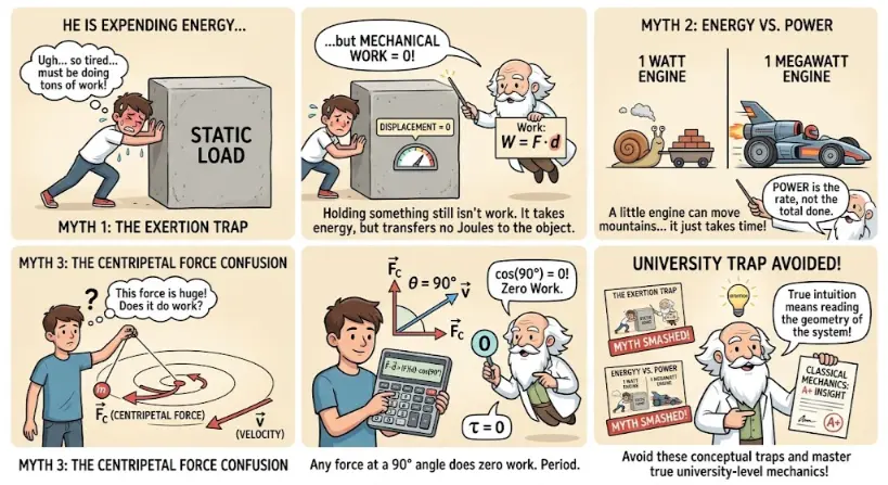
Does Physical Exhaustion Always Mean Mechanical Work is Done? No, physical exhaustion does not mean mechanical work is occurring. Holding an object stationary burns metabolic energy internally, but transfers zero mechanical energy to the object because its spatial displacement vector remains zero.
A conceptual map for identifying and correcting intuitive traps related to static force, power delivery, and non-parallel vector systems.
6. Thought-Provoking Conceptual Queries
To master alternating current regimes, students must look beyond static mechanical comparisons and investigate how the conservation of energy manifests across dynamic, time-varying electromagnetic boundaries. Unpack these complex scenario questions to audit your system intuition:
Question 1: The “Infinite Current” Paradox
If an ideal series RLC circuit is driven precisely at its resonant frequency (\(f_0\)), the inductive and capacitive reactances cancel out completely (\(X_L = X_C\)), reducing the net reactive impedance to zero. If the physical resistance \(R\) in the wires could also be cooled down to absolute zero to create a perfect superconductor, Ohm’s law suggests current would approach infinity (\(I = V/0 \rightarrow \infty\)). Why does this configuration not cause an instantaneous infinite energy explosion in real-world implementations?
Show Physical Resolution
The paradox breaks down because an “instantaneous” spike is physically impossible. Even if thermal resistance is zero, the circuit possesses a finite geometric inductance governed by its physical loop boundary layout. As current attempts to scale up, this residual self-inductance generates an immediate back-electromotive force (\(V = L \cdot \frac{di}{dt}\)) that limits the chronological rate of current rise.
Furthermore, as the current builds up, the system begins radiating energy away into the surrounding environment as electromagnetic waves. This radiation acts as a non-conservative damping mechanism known as radiation resistance, capping the peak current threshold and enforcing the conservation of energy.
Question 2: The Phase Displacement Real Power Deficit
An industrial assembly plant operates large electric induction motors that behave as massive inductors, creating an acute phase angle shift where current lags behind voltage. The utility grid delivers high apparent power (\(V_{\text{rms}} \cdot I_{\text{rms}}\)), yet the factory’s useful, true power consumption remains low. Where does the missing energy go, and why do utility companies penalize factories for running low power factor networks?
Show Physical Resolution
The energy is not lost; it is continuously sloshing back and forth twice per AC cycle between the power plant’s generators and the factory’s magnetic fields. This cycling energy is called reactive power.
While the factory does not burn this energy into permanent heat work, the extra current must still physically flow through the power grid’s transmission lines. Because real transmission lines have resistance, this sloshing current produces real heating waste (\(I^2 R\)) along the utility grid’s wires. Utility companies penalize low power factor configurations because they force the grid to build heavier lines and generate massive transmission losses to sustain a network that does not perform useful work at the destination.
Question 3: The Skin Effect and High-Frequency Blockades
If you drive a uniform solid cylindrical copper wire with high-frequency alternating current signals, the inner core of the conductor carries almost zero current, forcing the charge carriers to migrate strictly along the outer perimeter “skin” of the metal. What micro-scale field mechanisms cause this strange spatial displacement?
Show Physical Resolution
This phenomenon is driven entirely by Faraday’s Law of Induction. Alternating current running through a conductor establishes a time-varying magnetic field loop inside the wire’s own cross-section. These changing magnetic fields induce localized circulating current loops, known as eddy currents.
At the center of the wire, these eddy currents flow in the opposite direction of the primary current, canceling it out. Near the outer boundary, however, the eddy currents align parallel to the main current path, reinforcing it. As frequency escalates, this cancellation profile intensifies, confining charge transport to a thin superficial skin layer and drastically driving up the wire’s effective resistance.
7. Evolution of Circuit Paradigms: History, Engineering Frontiers, and the Quantum Future
The progression of circuit theory tracks a continuous technological journey from macroscopic mechanical systems to microscopic quantum states. Understanding these developmental milestones helps university-bound students contextualize modern engineering constraints.
The Historical Evolution
The foundation of modern networks began with the fierce “War of the Currents” in the late 19th century, pitting Thomas Edison’s Direct Current (DC) model against Nikola Tesla and George Westinghouse’s Alternating Current (AC) framework. While Edison’s DC system was highly effective for localized incandescent illumination, it lacked a mechanism to scale voltage up or down efficiently. This structural limitation meant power lines could only transmit energy about a mile before line resistance dissipated the current into useless heat.
Tesla’s insight was leveraging electromagnetic induction via the transformer. Because alternating fields can be stepped up to hyper-high voltage levels, utilities could slash transmission currents down to minimal values. Since line losses scale with the square of current (\(I^2 R\)), AC allowed power plants to transmit megawatts over hundreds of miles with negligible losses. This architectural victory standardized our modern centralized power grid.
Modern Contemporary Challenges
Today, contemporary circuit design has run head-first into rigid physical boundaries driven by extreme miniaturization. In modern integrated microchips, engineers pack billions of silicon field-effect transistors onto a chip the size of a fingernail, with feature dimensions scaling down below 5 nm. At these microscopic dimensions, circuits face two major crises:
Thermal Dissipation Constraints: Densely packed nanoscale pathways generate immense heat flux concentrations that can damage semiconductor structures if not managed with advanced cooling systems.
Parasitic Capacitive Leakage: When conductive traces are isolated by microscopic gaps only atoms wide, they form unintended, parasitic capacitors. High-frequency signals easily bleed across these gaps, distorting data profiles and corrupting signal integrity.
The Future Nature of Circuits
To bypass these silicon limitations, the next generation of circuit design is shifting toward radical new physical architectures. The most promising frontier is Integrated Silicon Photonics, which swaps electric charge carriers for photons. By channeling information via light beams through microscopic optical waveguides on a chip rather than moving electrons through copper traces, photonic circuits completely eliminate electrical resistance, generate zero Joule heating, and unlock transmission speeds bounded only by the speed of light.
Simultaneously, Quantum Circuit Architectures are moving from theory into commercial deployment. Instead of processing binary bits via classical on/off macroscopic switches, quantum processors manipulate quantum bits (qubits) using superconductive Josephson junctions. Operating at cryogenic temperatures near absolute zero, these loops sustain macro-scale quantum superposition and entanglement states. This shift redefines circuit logic, transforming standard nodes into complex probability field operations capable of handling computations that would choke a classical supercomputer.
8. Limits of the Classical Model
In basic circuit tutorials, we rely on the Lumped Element Model. This framework assumes that electrical effects occur instantly across perfectly discrete components (resistors, capacitors, inductors) connected by zero-resistance, zero-inductance virtual wires. This model simplifies network analysis, but it breaks down under two extreme conditions:
First, when the time-varying signal’s frequency scales into the gigahertz (\(\text{GHz}\)) or terahertz (\(\text{THz}\)) regimes, the operational electromagnetic wavelength (\(\lambda = c/f\)) shrinks until it matches or falls below the physical physical dimensions of the circuit board traces. Under these conditions, a wire can no longer be modeled as a simple equi-potential node. Instead, it must be treated as a distributed Transmission Line, where voltage wave pulses ripple along the path at finite speeds, generating signal reflections and phase delays if the line’s characteristic impedance is mismatched.
Second, when physical gate structures contract down to atomic scales, electrons ignore classical boundary walls entirely. Due to the wave-particle duality defined in quantum mechanics, electrons smoothly leak through insulating oxide barriers via quantum tunneling. This quantum leakage introduces parasitic leakage currents that bypass switch logic completely, requiring advanced non-classical materials (like sub-nanometer fin-FETs or carbon nanotube channels) to preserve system control.
9. Fermi Estimation Project
The Challenge: Estimate the total reactive energy temporarily stored inside the internal magnetic fields of all electrical distribution transformers across a large modern metropolis during peak air-conditioning utilization hours.
The Back-of-the-Envelope Approach: Let us model a metropolitan region hosting a population of roughly 4 × 10⁶ residents. Assuming an average density profile of 4 people per household yields a baseline grid of 1 × 10⁶ residential consumer nodes. During peak summer thermal loads, assume each household draws an average continuous power profile of roughly \(3\text{ kW}\), leading to a total city power requirement of:
Industrial grid step-down transformers generally carry a baseline inductance scale of roughly \(L \approx 50\text{ mH}\) (\(5 \times 10^{-2}\text{ H}\)) per sector array block. Operating on a standard utility profile where average branch current lines settle around \(I_{\text{rms}} \approx 200\text{ A}\), the peak energy stored within a single transformer’s inductive magnetic matrix tracks via:
Assuming each sector transformer handles approximately 50 neighborhood homes, the total transformer infrastructure array requires roughly 20,000 distributed sub-units. Multiplying this across our single unit storage baseline evaluates to:
This calculation demonstrates how Fermi estimation allows engineers to instantly translate consumer utilization data into large-scale infrastructure energy metrics without requiring granular, proprietary utility schematics.
10. Key Terms Glossary (Expanded)
Impedance (Z): The comprehensive complex vector parameter measuring total opposition to alternating current; incorporates real energy dissipation (resistance) and imaginary energy field storage (reactance). Measured in Ohms (\(\Omega\)).
Reactance (X): The frequency-dependent opposition to AC current generated strictly by energy storage inside electric fields (capacitive) or magnetic fields (inductive), without permanent energy loss.
Phasor: A complex vector that represents a sinusoidal signal’s magnitude and phase angle, rotating counterclockwise at a constant angular frequency (\(\omega\)) in a complex plane.
Power Factor: The scalar ratio of true power performed to apparent power delivered; mathematically evaluated as \(\cos(\phi)\), where \(\phi\) tracks the phase displacement angle.
Resonance: The network state where inductive and capacitive reactances are perfectly equal in magnitude and opposite in phase, maximizing branch currents in series lines or minimizing them in parallel arrays.
Skin Effect: The tendency of high-frequency alternating currents to distribute unevenly through a conductor, forcing current density to concentrate near the outer surface perimeter.
Admittance (Y): The reciprocal of impedance (\(Y = 1/Z\)), measuring how easily an alternating current flows through a network path. Measured in Siemens (\(\text{S}\)).
Quality Factor (Q): A dimensionless parameter that rates an oscillatory or resonant circuit’s efficiency, defined as the ratio of stored energy to energy dissipated per cycle.
Eddy Currents: Localized circulating loops of electric current induced within a conductor by a time-varying magnetic field, according to Faraday’s Law.
11. Numerical Problems and Solutions (Expanded Core Track)
1. An inductor has \(L = 0.20\text{ H}\) and is connected to an AC source of frequency \(50\text{ Hz}\). Find its inductive reactance.
Answer: The total circuit impedance magnitude is exactly 50 Ω. Because the inductive reactance exceeds capacitive parameters, the loop behaves with a net inductive phase character.
4. An AC circuit has \(V_{\text{rms}} = 120\text{ V}\) and impedance \(Z = 60\ \Omega\). Find \(I_{\text{rms}}\).
Answer: The resulting root-mean-square current tracking through the circuit equals exactly 2.0 A.
5. An AC circuit has \(V_{\text{rms}} = 230\text{ V}\), \(I_{\text{rms}} = 5.0\text{ A}\), and a power factor of \(\cos\phi = 0.80\). Find the true average power.
Solution: Compute the true, real-work dissipation power:
Answer: The circuit permanently converts energy into work at an average rate of 920 Watts.
Summary
AC circuits extend circuit physics from steady current to changing current. In AC, voltage and current vary with time, and their timing relationship becomes important.
Resistance describes ordinary opposition to current, while reactance describes frequency-dependent opposition caused by capacitors and inductors. Impedance combines these effects and determines the RMS current for a given AC voltage.
Final takeaway: AC circuits are governed not only by resistance, but also by frequency, reactance, impedance, and phase.