
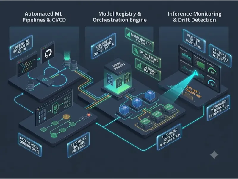
Interactive Quick Review: Traditional DevOps vs. MLOps
Why is traditional software DevOps insufficient for managing production machine learning applications?
Toggle Answer
Answer: Traditional DevOps manages code versioning and software build artifacts. MLOps must manage code, data versioning (DVC), and model parameters simultaneously. Furthermore, while software code remains deterministic post-deployment, ML model performance naturally degrades due to real-world data drift, requiring continuous telemetry, re-training pipelines, and model registry validation.
Architectural & Theoretical Deep Dives
1. Core Architectural Pillars of MLOps
A production-grade AI infrastructure comprises five essential subsystems:
- Feature Store: A centralized repository (e.g., Feast, Hopsworks) that processes, stores, and serves curated machine learning features for both offline batch training and low-latency online inference, preventing feature leakage between training and serving.
- Model Registry: A versioned catalog (e.g., MLflow, Weights & Biases) tracking trained model artifacts, hyperparameter lineage, performance evaluation metrics, and deployment stage transitions (Staging → Production → Archived).
- CI/CD/CT Pipelines: Continuous Integration (testing code and data quality), Continuous Deployment (packaging models into containerized microservices), and Continuous Training (CT) (automatically re-executing training jobs upon new data arrival or drift detection).
- Inference Engine & Orchestration: Serving platforms (e.g., Triton Inference Server, vLLM, TorchServe) orchestrated over Kubernetes clusters to manage GPU/CPU hardware acceleration, dynamic request batching, and horizontal autoscaling.
- Model Monitoring & Observability: Telemetry dashboards tracking operational infrastructure metrics (latency, GPU memory, throughput) alongside statistical data and concept drift metrics.
2. Detecting Model Degradation: Data Drift vs. Concept Drift
Statistical drift is the primary driver of performance decay in deployed ML models. Engineers classify drift into two distinct phenomena:
Data Drift (Covariate Shift): Occurs when the input feature distribution changes over time, while the conditional probability distribution of outputs given inputs remains constant:
$$P_{\text{train}}(X) \neq P_{\text{production}}(X), \quad \text{while } P(Y \mid X) \text{ remains fixed.}$$
Concept Drift: Occurs when the mathematical relationship between input features and target labels changes, even if the feature distribution $P(X)$ remains unchanged:
$$P_{\text{train}}(Y \mid X) \neq P_{\text{production}}(Y \mid X)$$
Statistical tests such as the Kolmogorov-Smirnov (KS) Test (for continuous features) and Population Stability Index (PSI) are regularly computed over windowed production data streams to trigger retrain events automatically.
3. Python Implementation: Population Stability Index (PSI) Drift Calculation
import numpy as np

from typing import Tuple


def calculate_psi(baseline: np.ndarray, target: np.ndarray, num_bins: int = 10) -> float:

    """

    Computes Population Stability Index (PSI) to detect data drift between baseline

    (training) and target (production) feature distributions.


    PSI Rules of Thumb:

    - PSI < 0.10: No significant distribution change.

    - 0.10 <= PSI < 0.25: Moderate drift; monitor closely.

    - PSI >= 0.25: Significant drift; trigger model retraining.

    """

    # 1. Determine bin edges using baseline distribution quantiles

    percentiles = np.linspace(0, 100, num_bins + 1)

    bin_edges = np.percentile(baseline, percentiles)


    # Adjust outer bounds to include all data points

    bin_edges[0] -= 1e-5

    bin_edges[-1] += 1e-5


    # 2. Calculate percentage of samples in each bin

    baseline_counts, _ = np.histogram(baseline, bins=bin_edges)

    target_counts, _ = np.histogram(target, bins=bin_edges)


    baseline_pct = baseline_counts / len(baseline)

    target_pct = target_counts / len(target)


    # Handle zero counts to prevent division by zero or log errors

    baseline_pct = np.where(baseline_pct == 0, 1e-4, baseline_pct)

    target_pct = np.where(target_pct == 0, 1e-4, target_pct)


    # 3. Compute PSI formula: sum((target% - baseline%) * ln(target% / baseline%))

    psi_value = np.sum((target_pct - baseline_pct) * np.log(target_pct / baseline_pct))

    return float(psi_value)


# Example Execution

np.random.seed(42)

training_features = np.random.normal(loc=0.0, scale=1.0, size=10000)

prod_features_normal = np.random.normal(loc=0.02, scale=1.01, size=5000)

prod_features_drifted = np.random.normal(loc=0.65, scale=1.20, size=5000)


psi_normal = calculate_psi(training_features, prod_features_normal)

psi_drift = calculate_psi(training_features, prod_features_drifted)


print(f"Normal Production Stream PSI: {psi_normal:.4f} (Status: OK)")

print(f"Drifted Production Stream PSI: {psi_drift:.4f} (Status: RETRAIN TRIGGERED)")
Interactive Quick Review: Blue/Green vs. Canary Deployments
Why are Canary deployments preferred over traditional Blue/Green cutovers when rolling out new machine learning models?
Toggle Answer
Answer: Blue/Green deployments switch 100% of live production traffic to a new service instantaneously. If a new ML model exhibits edge-case hallucinations, high latency, or unexpected inference failures, all users are impacted immediately. Canary deployments route a tiny fraction of live traffic (e.g., 5%) to the new model while monitoring latency, error rates, and predictive distributions, ensuring safe rollback before full traffic migration.
Taxonomy & Deployment Strategy Matrix
| Deployment Strategy | Traffic Routing Mechanism | Risk Profile | Primary Advantage | Infrastructure Requirements |
|---|---|---|---|---|
| Shadow Deployment | Replicates live requests to new model in parallel (outputs discarded) | Zero Risk (No user exposure) | Validates live production performance and latency under real load | 2× compute serving capacity |
| Canary Release | Incremental routing shift (e.g., 5% → 25% → 100%) | Low Risk | Limits blast radius of faulty models or latency regressions | Dynamic API Gateway / Service Mesh routing |
| A/B Testing | Splits users randomly between Model A and Model B | Moderate Risk | Measures real business metrics (click-through, conversion) | Experimentation & user session management engines |
| Blue/Green Cutover | Instantaneous switch from legacy environment to new environment | High Risk | Zero downtime deployment with instant rollback capabilities | Duplicate production serving clusters |
Applications, Trade-offs, & Future Outlook
Real-World Applications
- High-Frequency Financial Fraud Detection: Serving microsecond-latency model inference pipelines backed by online feature stores and automated drift retrain triggers.
- Automated Autonomous Vehicle Model Retraining: Ingesting terabytes of daily sensor telemetry, isolating high-loss driving edge cases, and orchestrating distributed GPU retraining pipelines.
- Enterprise LLM Inference Operations: Managing high-throughput vLLM cluster deployments with dynamic batching, PagedAttention VRAM management, and continuous prompt toxicity monitoring.
Engineering Trade-offs
The core challenge in MLOps is the Automation Overhead vs. Operational Complexity Dilemma. Setting up automated Continuous Training (CT) and complex Kubernetes infrastructure provides immense agility, but adds substantial cloud costs, pipeline maintenance overhead, and risk of automated retrain failures if bad data pollutes training pipelines.
Future Outlook & Emerging Research
Industry standards are shifting toward LLMOps—specialized infrastructure tailored to Large Language Models that manages prompt versioning, fine-tuning parameter adapters (LoRA), vector database retrieval indexing, and synthetic data generation pipelines. Concurrently, Declarative MLOps Frameworks are streamlining infrastructure code by unifying feature definitions, model training specifications, and deployment policies into single declarative configuration files.
Frequently Asked Questions
What is the difference between a Feature Store’s Online and Offline Store?
The Offline Store holds historical feature data optimized for high-throughput batch reads during model training (e.g., Parquet files on S3/Snowflake). The Online Store maintains only the latest feature values stored in low-latency key-value databases (e.g., Redis/DynamoDB) for sub-10ms retrieval during live inference.
What is Data Leakage in MLOps Pipelines?
Data leakage occurs when information from the target label or future test data inadvertently pollutes training features. Feature stores prevent leakage by enforcing strict point-in-time joins, ensuring features are calculated strictly using data available prior to the prediction timestamp.
How does Dynamic Batching improve Inference Throughput?
Inference servers aggregate individual real-time user requests arriving within a tiny time window (e.g., 5ms) into a single batched tensor pass. This maximizes GPU tensor core parallel processing utilization, vastly increasing overall system throughput.
What is Model Lineage and why is it essential for Compliance?
Model lineage records the exact chain of artifacts behind a deployed model: source code commit hash, training dataset version, feature transformation logic, hyperparameters, and evaluation metrics. Lineage tracking is mandatory under regulatory frameworks to audit model decisions.
End-of-Page Exercises & Assessment
Part 1: Review Questions
Q1: Define MLOps and state its primary goal in enterprise software engineering.
Answer: MLOps (Machine Learning Operations) is a discipline combining software DevOps, data engineering, and machine learning to automate the build, deployment, scaling, and monitoring lifecycle of ML models in production reliably and efficiently.
Q2: Explain the mathematical difference between Data Drift and Concept Drift.
Answer: Data Drift occurs when input feature distribution P(X) changes while conditional label distribution P(Y | X) remains fixed. Concept Drift occurs when the relationship between input features and labels P(Y | X) changes over time.
Q3: What role does a Model Registry perform within a CI/CD/CT pipeline?
Answer: A Model Registry stores and versions trained model binaries, hyperparameter metadata, and evaluation results, governing formal stage transitions (e.g., Staging to Production) and enabling instant rollback capabilities.
Q4: How does a Shadow Deployment work?
Answer: A Shadow Deployment mirrors live production request traffic to a candidate model in parallel. The candidate model executes inference and logs results for performance/latency evaluation, but its outputs are discarded without serving real users.
Q5: What is the Population Stability Index (PSI) threshold for triggering model retraining?
Answer: A PSI score below 0.10 indicates distribution stability; a PSI between 0.10 and 0.25 indicates moderate drift; a PSI score ≥ 0.25 indicates significant data drift that triggers automated retraining.
Part 2: Thought-Provoking Questions
Q1: Training-Serving Skew in Real-Time Recommender Systems
Scenario: An e-commerce engineering team trains a recommendation model using offline batch features computed over historical daily aggregates. When deployed live, conversion accuracy drops by 40% despite perfect offline test scores.
Analysis: This is an example of Training-Serving Skew. Offline training features were computed using complete end-of-day summaries, whereas the live online serving pipeline calculated features over incomplete real-time streaming windows. The fix is implementing a centralized Feature Store that enforces identical feature transformation logic and point-in-time correctness across both training batch queries and online key-value lookups.
Q2: Automated Retraining Loops Triggered by Corrupted Data Ingestion
Scenario: An automated Continuous Training (CT) pipeline triggers a retrain job whenever PSI drift exceeds 0.25. An upstream API change alters temperature sensor units from Celsius to Fahrenheit, spiking PSI to 0.85. The pipeline retrains and deploys a new model automatically, causing catastrophic system outages.
Analysis: The system suffered from unvalidated data pipeline feedback. Automated retraining loops must include strict Data Validation Checks (e.g., Great Expectations schema assertions) and mandatory Model Evaluation Gates. If the new model fails automated validation checks against a golden test benchmark, deployment must halt immediately with alert escalation to on-call engineers.
Part 3: Numerical Engineering Problems
Problem 1: Population Stability Index (PSI) Numerical Calculation
Question: Consider a single feature divided into 2 equal reference bins during training:
• Baseline Training Bin Fractions: Bin 1 = 50% (0.50), Bin 2 = 50% (0.50).
• Production Monitoring Bin Fractions: Bin 1 = 20% (0.20), Bin 2 = 80% (0.80).
Calculate the Population Stability Index (PSI) using the formula:
$$\text{PSI} = \sum \left( \text{Target}_i – \text{Baseline}_i \right) \times \ln\left( \frac{\text{Target}_i}{\text{Baseline}_i} \right)$$
Determine if the PSI score breaches the 0.25 retraining threshold.
Step-by-step Solution:
1. Bin 1 Calculation:
• Target1 – Baseline1 = 0.20 – 0.50 = -0.30.
• ln(Target1 / Baseline1) = ln(0.20 / 0.50) = ln(0.40) ≈ -0.9163.
• Term 1 = -0.30 × -0.9163 = 0.2749.
2. Bin 2 Calculation:
• Target2 – Baseline2 = 0.80 – 0.50 = +0.30.
• ln(Target2 / Baseline2) = ln(0.80 / 0.50) = ln(1.60) ≈ 0.4700.
• Term 2 = +0.30 × 0.4700 = 0.1410.
3. Sum PSI Terms:
• PSI = 0.2749 + 0.1410 = 0.4159.
Final Answer: The computed PSI is 0.4159. Because 0.4159 > 0.25, significant drift has occurred and automated retraining is triggered.
Problem 2: Inference Cluster GPU Sizing & Throughput Calculation
Question: A high-throughput model serving deployment handles a peak load of R = 1200 inference requests per second (RPS).
• A single GPU instance serves b = 16 batched requests per tensor pass.
• Each batched execution pass takes t = 40 ms (0.040 seconds).
1. Calculate the maximum throughput capability (RPS) of a single GPU instance.
2. Calculate the minimum number of GPU instances required to support peak load without queuing delays.
Step-by-step Solution:
1. Single GPU Throughput Calculation:
• Execution passes per second per GPU = 1.0 / 0.040 s = 25 passes/sec.
• Throughput per GPU = 25 passes/sec × 16 requests/pass = 400 RPS.
2. Compute Minimum GPU Instances Required:
• Instances required = Peak Load / Single GPU Throughput
• Instances required = 1200 RPS / 400 RPS = 3 GPU instances.
Final Answer: A single GPU instance serves 400 RPS; a minimum of 3 GPU instances are required to support peak production load.
AI Infrastructure & Governance Sub-Cluster
-
AI Safety, Ethics & Governance
Explore fairness metrics, bias mitigation algorithms, hallucination reduction, and regulatory compliance. -
Edge AI & Embedded Machine Learning
Learn TinyML techniques, model quantization, and optimization strategies for resource-constrained hardware. -
Artificial Intelligence Hub
Return to the main Artificial Intelligence overview covering machine learning paradigms, deep learning, and intelligent systems.
External Academic & Technical References
- MLOps: Continuous Delivery and Automation Pipelines in Machine Learning (MLOps.org) – Comprehensive industry architectural guide on MLOps standards.
- Hidden Technical Debt in Machine Learning Systems (Sculley et al., NeurIPS) – Seminal paper detailing architectural risks and operational maintenance costs in ML infrastructure.
- Kubernetes Production Container Orchestration Documentation – Official documentation on container deployment patterns and horizontal autoscaling.