
Optical amplifiers and signal loss are central ideas in modern fiber optic systems. Light can travel through an optical fiber for long distances, but it does not remain perfectly strong forever. Some light is absorbed, scattered, leaked at bends, lost at connectors, or weakened at splices. If the signal becomes too weak, the receiver may no longer distinguish the intended information clearly.
Optical amplifiers help solve this problem by strengthening light signals without first converting them into electrical signals. They are especially important in long-distance communication, submarine cables, high-capacity networks, and wavelength-division multiplexed systems where many optical channels travel through the same fiber.
This page belongs to the wider Fiber Optics cluster in Light and Optics. Earlier pages explain how fibers guide light by total internal reflection, how fiber modes and dispersion affect pulse spreading, and how optical fiber communication carries information using light. This page focuses on what happens when the signal weakens, how engineers estimate loss, and how optical amplifiers restore usable signal strength.
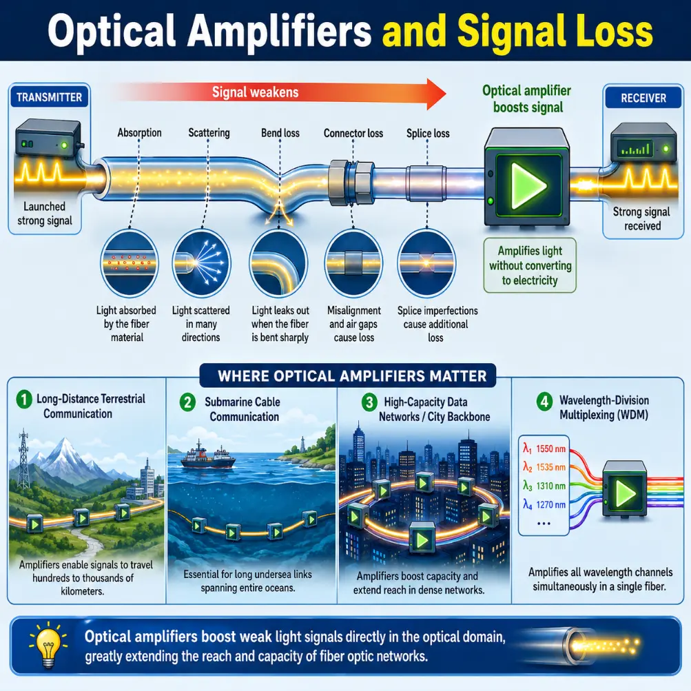
This illustration introduces optical amplifiers and signal loss in fiber optic systems. It shows a strong light signal launched into an optical fiber and gradually weakened by absorption, scattering, bend loss, connector loss, and splice loss. An optical amplifier then boosts the weakened light signal before it reaches the receiver. The lower panels show important applications where optical amplification matters, including long-distance terrestrial communication, submarine cable systems, high-capacity data networks, and wavelength-division multiplexed links carrying multiple optical channels through the same fiber.
Learning Pathway Within the Fiber Optics Module
Optical amplifiers and signal loss are best understood after students know how light is guided inside fibers and how information is carried by optical signals. Once those foundations are clear, students can study why signals weaken and how real networks keep them strong enough to be detected reliably. Use the roadmap below to navigate across the cluster levels:
Total Internal Reflection and Optical Fibers
Learn how light remains guided inside a fiber core when it meets the core-cladding boundary under the correct conditions.
Fiber Modes and Dispersion
Study how different guided modes, wavelengths, and propagation effects influence pulse spreading, bandwidth, and signal clarity.
Optical Fiber Communication
This page shows how optical fibers transmit information using light pulses, modulation, receivers, repeaters, and network systems.
Optical Amplifiers and Signal Loss
Current module. This page examines attenuation, scattering, absorption, bends, splices, connectors, link budgets, optical amplifiers, amplifier noise, and signal recovery.
Fiber Optic Sensors
This page explains how optical fibers can act as sensitive measuring devices for strain, temperature, vibration, pressure, chemical change, and structural monitoring.
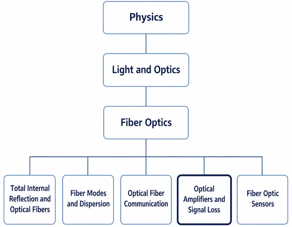
This tree chart shows the page hierarchy for the Fiber Optics cluster within Physics and Light and Optics. The parent topic, Fiber Optics, branches into five related subpages: Total Internal Reflection and Optical Fibers, Fiber Modes and Dispersion, Optical Fiber Communication, Optical Amplifiers and Signal Loss, and Fiber Optic Sensors. The Optical Amplifiers and Signal Loss page is highlighted to show the current position in the cluster, where students learn why optical signals weaken, how signal loss is estimated, and how optical amplifiers restore usable signal strength in fiber optic networks.
What Optical Amplifiers and Signal Loss REALLY Mean
A fiber optic system is not judged only by whether light can enter the fiber. It is judged by whether enough meaningful light reaches the receiver after travelling through the full link. The signal must survive distance, connectors, splices, bends, wavelength-dependent effects, and background noise. If the received signal becomes too weak or too noisy, information may be lost even though some light is still present.
Signal loss means that optical power decreases as light travels through the system. Some loss is unavoidable because real glass is not perfectly transparent. Some loss comes from installation and handling. Some loss comes from imperfect connections. The engineer’s task is not to eliminate all loss, but to understand it, control it, and design enough margin so that the receiver still works reliably.
An optical amplifier is a device that increases the power of an optical signal. Instead of detecting the signal, converting it into an electrical waveform, amplifying it electronically, and converting it back into light, an optical amplifier strengthens the light directly. This is one reason optical amplifiers are so important in long-distance, high-capacity fiber networks.
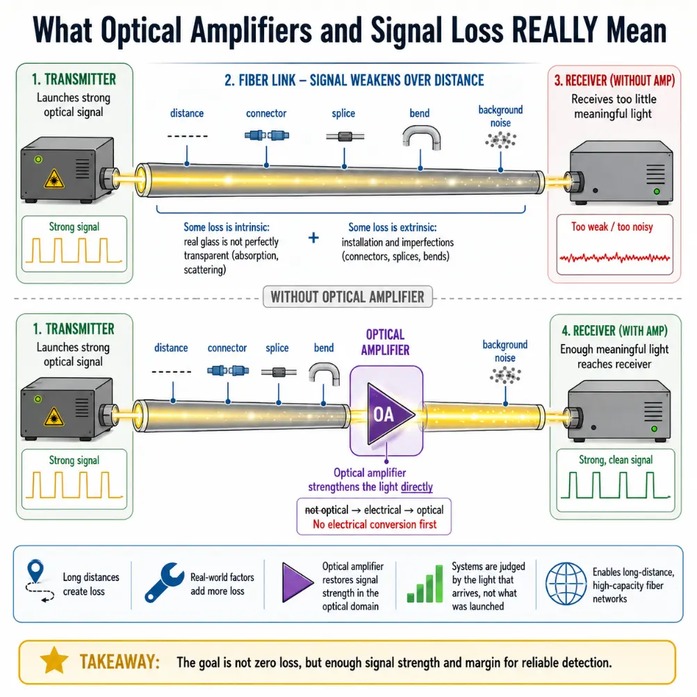
This illustration explains the practical meaning of optical amplifiers and signal loss in a fiber optic link. It compares a signal that becomes too weak or noisy after travelling through distance, connectors, splices, bends, and background noise with a signal that is strengthened by an optical amplifier before reaching the receiver. The diagram emphasizes that some loss is unavoidable, while some loss comes from installation and handling. It also shows that an optical amplifier restores signal strength directly in the optical domain, without first converting the light into an electrical signal. The key idea is that the goal is not zero loss, but enough signal strength and system margin for reliable detection.
Theoretical Framework: Attenuation Scaling Laws, Decibel Arithmetic, and Laser Gain Physics
To analyze power drop and link gains with total undergraduate physical rigor, students must master the exponential scaling laws and quantum mechanics governing light amplification.
Exponential Attenuation Scaling Laws
As photons propagate down a silica fiber core, their power loss is governed by an exponential decay relationship. This attenuation arises primarily from a combination of Rayleigh scattering and localized material absorption. The remaining optical power P at a distance L along the waveguide can be expressed as:
$$P(L) = P_0 e^{-\alpha_e L}$$Where P0 represents the initial input power launched by the transmitter and αe matches the attenuation coefficient in nepers per unit distance. In telecommunication fields, engineers scale this exponential drop into a base-10 logarithmic system to simplify link planning into linear decibel equations:
$$\alpha_{\text{dB/km}} = \frac{10}{L} \log_{10}\left(\frac{P_0}{P(L)}\right)$$This logarithmic scaling allows for direct subtraction of losses across a cascade of fiber links, connectors, and splices. To baseline optical intensities across hardware frameworks, absolute powers are calculated in units of dBm, which normalize measurements against a standard reference floor of 1 mW:
$$\text{Power in dBm} = 10 \log_{10}\left(\frac{P_{\text{mW}}}{1 \text{ mW}}\right)$$Erbium Laser Core Population Inversion Mechanics
Erbium-doped fiber amplifiers (EDFAs) restore weak optical signals directly by driving a population inversion inside a core segment doped with trivalent erbium ions (Er3+). A local pump laser operating at a high-energy band (typically 980 nm or 1480 nm) excites the ground-state ions from the 4I15/2 level up to elevated energy bands. The ions undergo rapid non-radiative decay to settle into a long-lived metastable state, marked 4I13/2.
When weak 1550 nm input signals cross this energized core segment, they stimulate the excited ions to drop back down to the ground state. This radiative decay releases identical photons that share the exact phase, frequency, and polarization profiles of the passing wave, producing a coherent increase in power:
$$G(\lambda) = e^{\left[\sigma_e(\lambda)N_2 – \sigma_a(\lambda)N_1\right]L_{\text{doped}}}$$Where σe and σa are the emission and absorption cross-sections at wavelength λ, N2 is the excited population density, N1 represents the ground-state ion density, and Ldoped is the total physical length of the doped fiber segment.
Why Optical Signals Become Weak
Optical signals weaken because a fiber link is a real physical system. Light interacts with glass, coatings, connectors, bends, splices, and components. Each interaction may remove a small amount of power from the useful guided signal.
Absorption: Occurs when optical energy is taken up by the material of the fiber or by impurities inside the glass. Some of the light energy is converted into other forms, such as heat. Modern optical fibers are carefully manufactured to reduce absorption, but no real material is perfectly transparent at every wavelength.
Scattering: Occurs when small variations in the glass redirect some light away from the useful guided direction. Rayleigh scattering is especially important in optical fibers. It is one reason shorter wavelengths usually suffer more loss than longer wavelengths in silica fibers.
Bending Loss: Occurs when a fiber is bent too sharply. The guided light can no longer remain fully confined in the core, and some energy leaks into the cladding or surrounding material. This is why fiber cables have minimum bend-radius recommendations.
Connector Loss: Occurs where two fiber ends meet through a connector. Dirt, scratches, air gaps, poor alignment, or damaged end faces can reduce the amount of light coupled from one fiber into the next. Clean connector inspection is one of the most important maintenance practices in fiber optics.
Splice Loss: Occurs where two fibers are joined permanently or semi-permanently. A good fusion splice may have very low loss, but poor alignment, different fiber types, contamination, or imperfect heating can increase loss.
Optical Link Budgets and System Margin
An optical link budget is a calculation that checks whether enough optical power will reach the receiver. It compares the transmitter output power, total losses, amplifier gains, receiver sensitivity, and safety margin. When powers, losses, and gains are expressed in dBm and dB, the calculation uses simple addition and subtraction:
$$P_{\text{received}} = P_{\text{transmitted}} – \text{total losses} + \text{total gains}$$System Margin: Extra allowance included to keep the link reliable even when conditions are not perfect. It accounts for ageing, repairs, future splices, temperature effects, connector wear, measurement uncertainty, and unexpected losses.
Receiver Sensitivity: The minimum optical power the receiver needs to detect the signal correctly. If the received power falls below this value, the bit error rate may become too high for standard use.
Power Penalty: Extra optical power required because of dispersion, noise, nonlinear effects, imperfect extinction ratio, or other signal-quality problems. A link may have enough average power but still perform poorly if the signal shape is degraded.
Architectures of Optical Amplification Hardware
Different hardware configurations exploit specific quantum or material behaviors to scale light signal intensities directly:
Erbium-Doped Fiber Amplifiers (EDFA): Utilize a length of silica fiber core infused with trivalent erbium ions. When energized by an external pump laser, the medium delivers high-gain, low-noise amplification across the entire 1550 nm telecommunication transmission window, allowing many channels to be boosted together without distortion.
Raman Amplifiers: Exploit a nonlinear optical behavior known as stimulated Raman scattering. Energy transfers directly from high-power pump lasers to data waves along the transmission fiber itself. This creates distributed gain profiles that improve noise margins over long distances.
Semiconductor Optical Amplifiers (SOA): Utilize a compact, electrically driven semiconductor chip structure to form a gain region. While more prone to nonlinear distortions than fiber amplifiers, their compact size makes them ideal for localized routing switches and integrated photonic circuits.
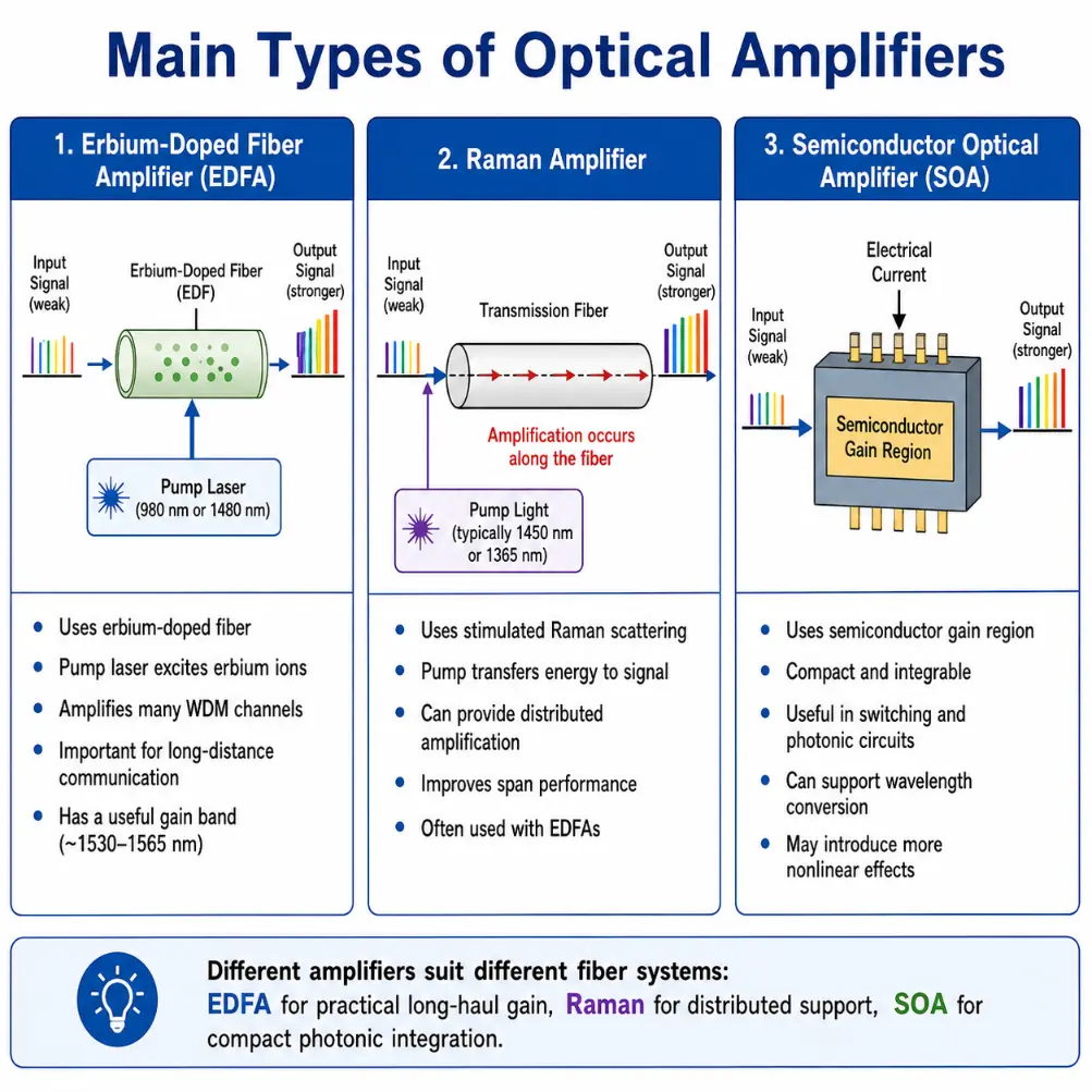
This educational illustration presents the main types of optical amplifiers used in fiber optic systems. It compares the erbium-doped fiber amplifier (EDFA), the Raman amplifier, and the semiconductor optical amplifier (SOA). The EDFA panel shows a weak input signal passing through erbium-doped fiber, where pump laser energy excites erbium ions and amplifies many wavelength-division multiplexed channels across a useful gain band. The Raman amplifier panel shows amplification occurring along the transmission fiber through stimulated Raman scattering, with pump light transferring energy to the signal and improving span performance. The SOA panel shows a semiconductor gain region amplifying a weak input signal, highlighting its compact size, suitability for photonic integration, and use in switching, signal processing, and wavelength conversion. Together, the diagram helps students understand that different optical amplifiers are suited to different fiber system needs.
Operational Constraints: Noise Accumulation and Gain Saturation
Optical amplifiers are highly effective, but they add new variables that must be managed to keep links performing reliably:
Amplified Spontaneous Emission (ASE): Excited ions inside a core segment can drop down to their ground state randomly instead of waiting for a passing signal photon. This spontaneous emission is amplified along the line, creating background noise that can obscure weak data signals. This degradation is measured by the amplifier’s noise figure.
Gain Saturation Limits: As the incoming signal power increases, it depletes the pool of excited ions faster than the pump laser can re-energize them. This causes the amplifier gain to drop. In multi-channel networks, gain saturation must be carefully balanced so that strong channels do not drain power away from weaker ones.
Gain Tilt and Non-Uniformity: Amplifiers do not boost every wavelength equally across their gain band. Left unmanaged, small variations in gain accumulate over long distances, causing some channels to overpower others. Engineers use gain-flattening filters to balance power levels across the entire spectrum.
Optical Amplifier Placement Strategies
The same optoelectronic hardware unit is named differently based on where it is integrated along a fiber optic link:
Booster Amplifier: Positioned directly after the transmitter module. It increases initial launch power levels to push signals safely across long spans before they fade toward the background noise floor.
Inline Amplifier: Positioned at regular intervals (typically every 80 to 100 km) along long terrestrial or transoceanic links. It balances out span losses without needing costly optical-electrical-optical conversions.
Pre-Amplifier: Positioned directly ahead of the optical receiver module. It boosts weak incoming light fields above the thermal noise floor of the detector diode, maximizing detection accuracy.
Applications of Optical Amplifiers and Loss Management
Optical amplifiers and loss management are important wherever optical signals must remain strong, clean, and interpretable over distance or through complex networks.
Long-Haul Communications
Terrestrial and metropolitan core networks deploy inline EDFAs to maintain signal strength across major infrastructure networks.Submarine Cable Systems
Transoceanic links integrate undersea amplification modules to transmit high-speed data across oceans with low error rates.WDM High-Capacity Links
Wavelength-division multiplexed lines use gain-flattened amplifiers to boost dozens of unique data channels simultaneously down a single fiber.Data Centre Interconnects
Dense optical links use strict power management and precise connector specifications to handle massive data routing demands with minimal loss.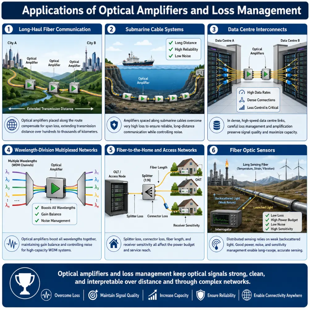
This infographic presents the main applications of optical amplifiers and loss management in fiber optic systems. It shows long-haul terrestrial communication, where amplifiers placed along the route compensate for span loss and extend transmission distance. It also illustrates submarine cable systems, where carefully spaced amplification supports reliable communication across oceans while controlling noise. Additional panels show data centre interconnects, where dense high-speed fiber links require strict loss control, and wavelength-division multiplexed networks, where one amplifier can strengthen many wavelength channels while maintaining gain balance and managing noise. The infographic also includes fiber-to-the-home and access networks, where splitter loss, connector loss, fiber length, and receiver sensitivity shape the power budget, and fiber optic sensors, where weak backscattered light in distributed sensing requires careful management of power, noise, and sensitivity. Together, these examples show that optical amplifiers and loss management are essential wherever optical signals must remain strong, clean, and interpretable.
Common Conceptual Misunderstandings
The Signal Perfection Illusion
Misconception: Passing a weak, distorted light pulse through an optical amplifier removes noise and fixes dispersion errors. Reality: Amplifiers only boost optical power; they do not reshape or retime waves. Unmanaged noise and dispersion are amplified along with the signal, meaning a regenerator may be needed to clean up heavily distorted pulses.The Unlimited Power Fallacy
Misconception: Simply increasing launch laser powers to maximum is always the best way to bypass fiber attenuation constraints. Reality: Excessively high power densities trigger non-linear optical effects like four-wave mixing and stimulated Brillouin scattering, which degrade performance and can permanently damage the fiber faces.Interactive Quick Checks
Quick Check: Optical Amplifiers and Signal Loss
1. If a fiber link has signal loss, does it mean all light has disappeared?
No. Signal loss means the optical power has decreased. Some light may still reach the receiver, but it may not be strong enough or clean enough for reliable detection.
2. Why are dB values convenient in fiber link budgets?
They make link calculations easier because losses and gains can be added or subtracted directly when powers are expressed in dBm and losses or gains are expressed in dB.
3. What is the main difference between an optical amplifier and an electronic repeater?
An optical amplifier strengthens the light directly. An electronic repeater converts the light into an electrical signal, processes it, and then transmits a new optical signal.
Numerical Practice: Link Budget Math
Numerical Problems and Solutions
Worked Example 1: A transmission fiber features an attenuation constant of 0.25 dB/km. Find the total fiber power loss over a length of 40 km.
Multiply the linear attenuation rate by the total link distance:
$$\text{Fiber Loss} = \alpha \times L = 0.25\text{ dB/km} \times 40\text{ km} = 10.0\text{ dB}$$Answer: The total fiber attenuation loss evaluates to exactly 10 dB.
Worked Example 2: A fiber span covers 30 km with an attenuation of 0.2 dB/km, four connectors each introducing 0.5 dB of loss, and six fusion splices each introducing 0.1 dB of loss. Calculate the total link loss.
Calculate and sum each individual loss component:
$$\text{Fiber Attenuation} = 0.2\text{ dB/km} \times 30\text{ km} = 6.0\text{ dB}$$
$$\text{Connector Losses} = 4 \times 0.5\text{ dB} = 2.0\text{ dB}$$
$$\text{Splice Losses} = 6 \times 0.1\text{ dB} = 0.6\text{ dB}$$
$$\text{Total Loss} = 6.0\text{ dB} + 2.0\text{ dB} + 0.6\text{ dB} = 8.6\text{ dB}$$Answer: The total link power loss is exactly 8.6 dB.
Worked Example 3: A laser diode launches an initial power of 2 dBm into a fiber link. If the total calculated link loss tracks at 14 dB, determine the absolute power reaching the receiver.
Subtract the total decibel loss from the initial normalized transmitter power:
$$P_{\text{received}} = P_{\text{transmitted}} – \text{Total Loss} = 2\text{ dBm} – 14\text{ dB} = -12\text{ dBm}$$Answer: The received power tracks at exactly −12 dBm.
Worked Example 4: A weak optical wavefront hits an EDFA core segment at an intensity of −18 dBm. If the amplifier configuration provides 20 dB of active gain, determine the output power.
Add the active amplifier gain directly to the incoming input signal power:
$$P_{\text{out}} = P_{\text{in}} + \text{Gain} = -18\text{ dBm} + 20\text{ dB} = 2\text{ dBm}$$Answer: The amplifier output power is exactly 2 dBm.
Worked Example 5: A photodiode receiver sensitivity threshold requires at least −20 dBm to process data. If the calculated received power tracks at −15 dBm, determine the link margin.
Subtract the minimum required threshold power from the actual received power:
$$\text{Margin} = P_{\text{received}} – P_{\text{minimum}} = -15\text{ dBm} – (-20\text{ dBm}) = 5\text{ dB}$$Answer: The available link power safety margin is exactly 5 dB.
Problem 1: An optical line features an attenuation rate of 0.3 dB/km. Find the absolute fiber loss encountered across a length of 25 km.
Multiply the attenuation coefficient by the transmission line length:
$$\text{Loss} = \alpha \times L = 0.3\text{ dB/km} \times 25\text{ km} = 7.5\text{ dB}$$Answer: The total fiber attenuation loss scales to 7.5 dB.
Problem 2: A transmitter launches 5 dBm into a long span. If the total network path loss is 18 dB, find the received power.
Subtract the path loss directly from the launch power parameter:
$$P_{\text{received}} = 5\text{ dBm} – 18\text{ dB} = -13\text{ dBm}$$Answer: The received signal power is exactly −13 dBm.
Problem 3: An input signal measuring −22 dBm enters an active gain module. If the amplifier provides 17 dB of gain, calculate the final output power.
Add the decibel gain to the input power value:
$$P_{\text{out}} = -22\text{ dBm} + 17\text{ dB} = -5\text{ dBm}$$Answer: The output power is exactly −5 dBm.
Problem 4: A fiber network links over 50 km with an attenuation constant of 0.22 dB/km, two connectors with a loss of 0.4 dB each, and ten splices with a loss of 0.08 dB each. Determine the total link loss.
Sum all contributing loss factors line-by-line:
$$\text{Fiber Attenuation} = 0.22\text{ dB/km} \times 50\text{ km} = 11.0\text{ dB}$$
$$\text{Connector Disruption} = 2 \times 0.4\text{ dB} = 0.8\text{ dB}$$
$$\text{Splice Imperfections} = 10 \times 0.08\text{ dB} = 0.8\text{ dB}$$
$$\text{Total Loss} = 11.0\text{ dB} + 0.8\text{ dB} + 0.8\text{ dB} = 12.6\text{ dB}$$Answer: The combined total link loss scales to exactly 12.6 dB.
Problem 5: A photodiode receiver sensitivity measures −24 dBm. If the processed received power evaluates to −19 dBm, find the safety margin.
Subtract the required sensitivity threshold from the actual power value:
$$\text{Margin} = -19\text{ dBm} – (-24\text{ dBm}) = 5\text{ dB}$$Answer: The link operating margin is exactly 5 dB.
Problem 6: A long-distance fiber link features a passive path loss of 28 dB. If an integrated inline amplifier provides 20 dB of active gain, calculate the net loss across the span.
Subtract the amplifier gain value from the initial passive link loss:
$$\text{Net Loss} = 28\text{ dB} – 20\text{ dB} = 8\text{ dB}$$Answer: The net system loss after inline amplification is exactly 8 dB.
Problem 7: An optical pulse enters a lossy channel where its power is reduced from 1.0 mW down to 0.01 mW. Calculate the absolute link loss in decibels.
Apply the decibel conversion ratio formula:
$$\text{Loss in dB} = 10 \log_{10}\left(\frac{P_{\text{in}}}{P_{\text{out}}}\right) = 10 \log_{10}\left(\frac{1.0\text{ mW}}{0.01\text{ mW}}\right)$$
$$\text{Loss in dB} = 10 \log_{10}(100) = 10 \times 2 = 20\text{ dB}$$Answer: The absolute link power loss is exactly 20 dB.
Problem 8: A network design requires an intensity of at least −18 dBm at the receiver diode. If the transmitter launches 3 dBm and the total passive loss across the path is 26 dB, determine the minimum amplifier gain needed to close the link budget.
First, determine the unamplified power reaching the receiver:
$$P_{\text{unamplified}} = 3\text{ dBm} – 26\text{ dB} = -23\text{ dBm}$$Calculate the difference between the target minimum power and this unamplified level:
$$\text{Required Gain} = P_{\text{target}} – P_{\text{unamplified}} = -18\text{ dBm} – (-23\text{ dBm}) = 5\text{ dB}$$Answer: At least 5 dB of active optical amplifier gain is required to satisfy the basic link budget.
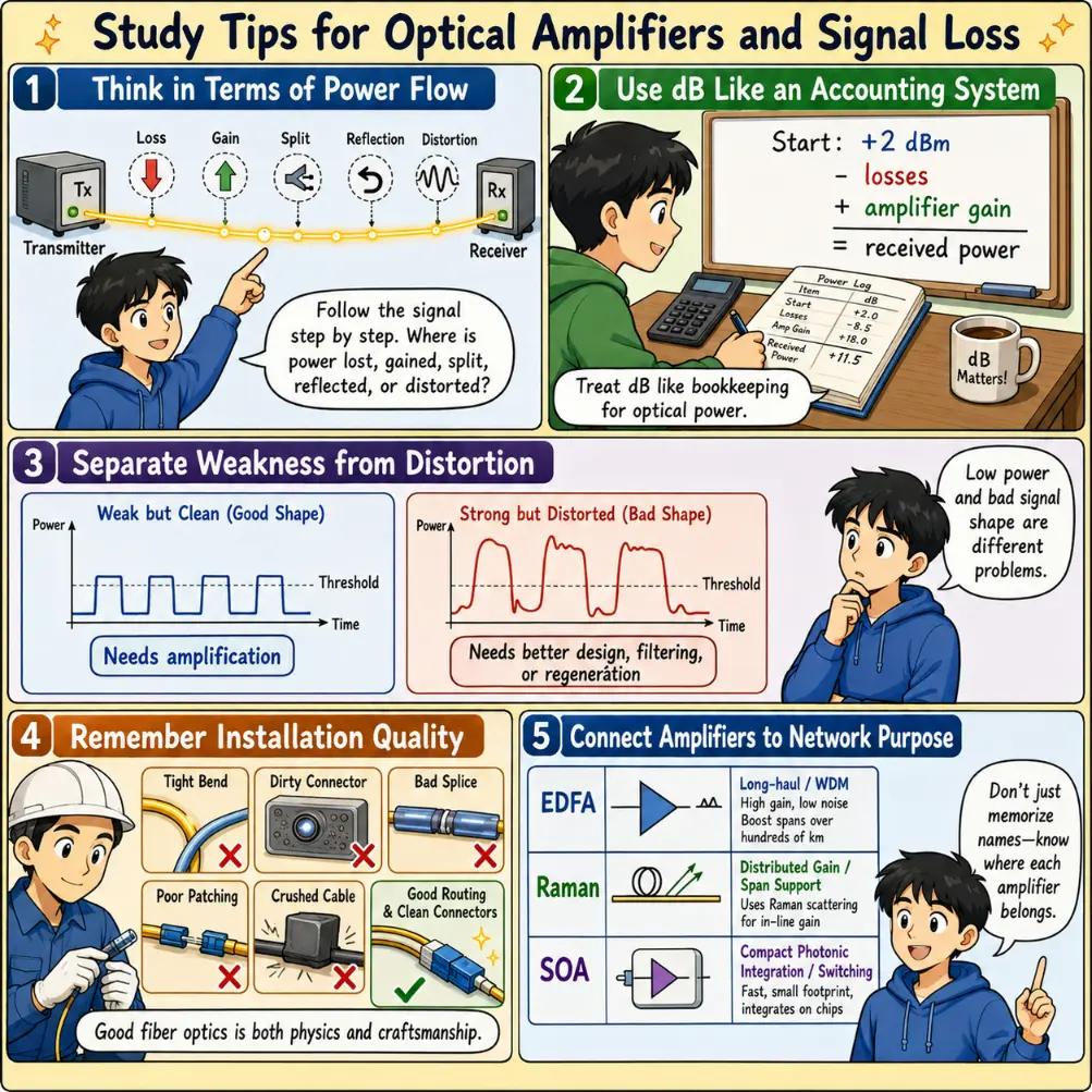
Study Tips
Follow the Power Flow: Track the signal from transmitter to receiver. At each step, ask whether power is lost, gained, split, reflected, or distorted.
Use dB Like an Accounting System: Treat dB calculations like a balance sheet. Start with transmitter power in dBm, subtract losses in dB, add amplifier gains in dB, and compare the final value with receiver sensitivity.
Separate Weakness from Distortion: A weak signal needs power recovery. A distorted signal may need dispersion management, filtering, regeneration, or better system design. Amplification alone does not solve every problem.
Remember Installation Quality: Many practical losses come from ordinary handling: tight bends, dirty connectors, bad splices, poor patching, or crushed cables. Good fiber optics is both physics and craftsmanship.
Key Terms
- Attenuation
- The gradual reduction of absolute optical power density as a light wave propagates through a waveguide channel, measured in dB/km.
- Decibel (dB)
- A logarithmic unit used to express the ratio between two optical power values.
- dBm
- An absolute logarithmic unit of power normalized against a reference floor baseline of exactly 1 mW.
- Link Budget
- The cumulative mathematical balancing of all gains, losses, and power margins across an entire optical link path.
- Erbium-Doped Fiber Amplifier (EDFA)
- An active fiber core component injected with erbium ions that uses a local pump laser to boost signals inside the 1550 nm window.
- Amplified Spontaneous Emission (ASE)
- The structural background noise generated inside an optical amplifier by excited ions dropping down to lower energy levels randomly.
- System Margin
- A dedicated power buffer built into link budgets to ensure reliable communication despite cable aging, scratches, or unexpected repairs.
External References
The Fiber Optic Association — Operational guidelines outlining connector cleaning protocols, fusion splicing methods, and optical power meter test setups.
RP Photonics Encyclopedia — Technical analyses outlining the quantum behaviors of erbium fiber lines, Raman scattering physics, and gain saturation limits.
Optica Publishing Group — Research databases tracking developments in dense wavelength division multiplexing and ultra-low-noise pre-amplifiers.
IEEE Xplore Digital Library — Engineering whitepapers detailing long-range transoceanic link budgets and semiconductor optical amplifier switching speeds.
International Telecommunication Union — Global telecommunication frameworks outlining standard baseline specifications for optical amplifiers and linear attenuation metrics.
Summary
Optical fiber signals become weaker as they travel through real fiber links. Loss can come from fiber attenuation, absorption, scattering, bending, connectors, splices, splitters, and other components. Engineers estimate these effects using decibels and link budgets so that enough optical power reaches the receiver. Optical amplifiers restore signal power while the signal remains in optical form. Important amplifier types include erbium-doped fiber amplifiers, Raman amplifiers, and semiconductor optical amplifiers. Amplifiers may be used as boosters, inline amplifiers, or pre-amplifiers depending on where they are placed in the link. Good fiber system design is not only about making the signal stronger. It also requires control of amplifier noise, gain saturation, wavelength balance, dispersion, nonlinear effects, connector quality, splice quality, bend radius, and system margin. A reliable fiber optic link is therefore a careful balance between light, materials, devices, installation, and engineering judgement.
Reflection Question
If an optical amplifier can make a weak signal stronger but cannot automatically remove noise or distortion, how should engineers decide when to amplify, when to regenerate, and when to redesign the fiber link itself?