
Introduction to Linear Algebra
Linear algebra studies vectors, matrices, and systems of linear equations. These mathematical tools are used throughout science, engineering, economics, computer graphics, robotics, artificial intelligence, and data science. Many complex systems can be described as relationships between multiple variables, and linear algebra provides efficient methods for analysing and solving such systems.
This primer introduces the fundamental ideas of linear algebra through geometric intuition, clear explanations, and simple numerical examples. The goal is to provide a foundation that prepares students for further study in mathematics, physics, engineering, economics, and computing.
Curriculum Navigation & Topic Cluster
Explore related advanced modules across our quantitative curriculum roadmap to deepen your knowledge of applied mathematics, system modeling, and data science:
Deep Learning & AI
Deep Learning Primer: Learn how multi-dimensional tensors, weight matrices, and vector transformations drive deep neural network architectures and backpropagation algorithms.
Data Analysis & Statistics
Data Analysis Foundations: Understand how covariance matrices, singular value decomposition (SVD), and principal component analysis (PCA) simplify high-dimensional datasets.
Computer Vision
Computer Vision Principles: Discover how 2D/3D affine transformations, projection matrices, and image filtering operations process visual spatial data.
Signal Processing
Digital Signal Processing: Explore how orthogonal basis vectors, Fourier transform matrices, and linear filtering process continuous and discrete signals.
Control Systems Engineering
Control Systems Modeling: Study state-space representations where matrix differential equations and eigenvalue stability determine system dynamics.
Robot Kinematics
Robot Kinematics & Dynamics: Apply homogeneous rotation matrices and Jacobian vector spaces to solve forward and inverse manipulator motion.
Quantum Computing
Quantum Computing Fundamentals: Examine how quantum qubits exist as complex state vectors and quantum gates act as unitary matrix operators.
Structural Engineering
Structural Matrix Analysis: Analyze structural framework stability and resonance modes using finite element stiffness matrices and natural frequency eigenvalues.
Vectors
A vector is a quantity that has both magnitude and direction. In geometry, vectors are represented as arrows in a coordinate system. For example, a movement of 3 units horizontally and 4 units vertically can be represented by the vector
The magnitude of the vector can be calculated using the Pythagorean theorem:
Vectors are widely used to represent displacement, velocity, force, and numerical data in many fields.
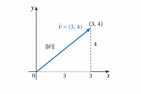
This diagram illustrates a vector v = (3,4) drawn from the origin to the point (3,4) on a Cartesian coordinate system. The dashed horizontal and vertical lines show how the vector can be decomposed into its components along the x-axis and y-axis. The horizontal component has magnitude 3 and the vertical component has magnitude 4, forming a right triangle that visually explains how vectors combine direction and magnitude in linear algebra.
Vector Addition
Vectors can be added by adding their corresponding components.
B = (3, 1)
A + B = (2 + 3, 4 + 1) = (5, 5)
Geometrically, this can be visualised using the tip-to-tail method.
Video Illustration: Vector Addition Methods
The following short video demonstrates three common methods used to add vectors: the tip-to-tail method, the parallelogram method, and the component method. These approaches help students visualize how vectors combine both geometrically and algebraically.
The demonstration shows how vectors can be represented graphically on a coordinate plane and how their components along the x and y directions determine the final resultant vector.
Watch the video here:
Vector Addition using Tip-to-Tail, Parallelogram, and Component Methods
The methods illustrated in the video form an important foundation for later topics in linear algebra, including vector operations, matrix transformations, and geometric interpretations used in physics, computer graphics, robotics, and data science.
Vector Subtraction
Vector subtraction measures the difference between two vectors.
B = (2, 1)
A – B = (5 – 2, 3 – 1) = (3, 2)
Dot Product
The dot product combines two vectors to produce a scalar quantity.
A · B = (2)(4) + (3)(1) = 8 + 3 = 11
The dot product is related to the angle between vectors:
If the dot product equals zero, the vectors are perpendicular (orthogonal).
Cross Product
The cross product is defined for three-dimensional vectors and produces a vector that is perpendicular to both input vectors. One convenient way to compute the cross product is to use a determinant involving the unit vectors i, j, k.
Suppose
The cross product can be written as the determinant evaluation:
Expanding the determinant gives:
u × v = [(-1)(-4) – (3)(7)] i – [(2)(-4) – (3)(5)] j + [(2)(7) – (-1)(5)] k
u × v = (4 – 21) i – (-8 – 15) j + (14 + 5) k
u × v = -17 i + 23 j + 19 k = (-17, 23, 19)
The resulting vector is perpendicular to both u and v.
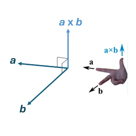
This diagram illustrates the geometric meaning of the cross product in three-dimensional space. Two vectors, a and b, originate from the same point and define a plane. The resulting vector a × b points perpendicular to the plane formed by a and b, indicating both the orientation and magnitude of the cross product according to the right-hand rule.
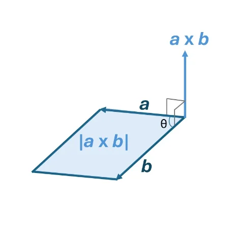
This diagram illustrates another geometric meaning of the cross product in three-dimensional space. Two vectors, a and b, originate from the same point and form an angle θ between them. Together they define a parallelogram whose area is equal to the magnitude of the cross product, |a × b|.
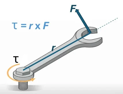
This diagram illustrates the physical meaning of the cross product in rotational mechanics. A wrench is used to turn a bolt, which acts as the pivot point. The vector r represents the position vector from the pivot to the point where the force is applied. The applied force F acts at an angle to the wrench, producing a torque τ that causes the bolt to rotate. The torque is determined by the cross product τ = r × F, meaning its magnitude depends on the length of the lever arm r, the magnitude of the force F, and the sine of the angle between them.
Matrices
A matrix is a rectangular arrangement of numbers organised in rows and columns. Matrices allow large systems of equations to be represented compactly.
Example Matrices: Consider the following matrices of different dimensions.
B = [ 5 1 ; 2 0 ] (2 × 2)
C = [ 2 3 1 ] (1 × 3)
D = [ 1 4 2 ; 0 3 5 ] (2 × 3)
E = [ 2 1 ; 3 0 ; 4 2 ] (3 × 2)
Matrix Addition: Two matrices can be added only if they have the same dimensions.
For example, matrices A and B are both 2×2 matrices, so their sum is defined:
However, matrices A and D cannot be added because their dimensions differ (2×2 versus 2×3).
Matrix Subtraction: Subtraction follows the same rule as addition: the matrices must have identical dimensions.
Matrix Multiplication: Matrix multiplication is defined when the number of columns of the first matrix equals the number of rows of the second matrix.
For example, matrix D is a 2×3 matrix and matrix E is a 3×2 matrix. Since the inner dimensions match (3 = 3), the product DE can be computed. The result will be a 2×2 matrix.
DE = [ (1×2 + 4×3 + 2×4) (1×1 + 4×0 + 2×2) ; (0×2 + 3×3 + 5×4) (0×1 + 3×0 + 5×2) ]
DE = [ (2 + 12 + 8) (1 + 0 + 4) ; (0 + 9 + 20) (0 + 0 + 10) ] = [ 22 5 ; 29 10 ]
Notice that the multiplication uses rows from the first matrix and columns from the second matrix. Because of this structure, matrix multiplication is generally not commutative, meaning that DE is not necessarily equal to ED.
Transpose of a Matrix: The transpose of a matrix is obtained by interchanging its rows and columns.
For example, the transpose of matrix D is:
A 2×3 matrix becomes a 3×2 matrix after transposition.
Systems of Linear Equations
Example System: Consider the following system of linear equations:
x – y = 1
We solve this system using three distinct algebraic methods.
Method 1: Substitution
From the second equation (x – y = 1), solve for x: x = y + 1. Substitute into the first equation:
Substitute back into x = y + 1 ⇒ x = 1 + 1 = 2
Solution: (x, y) = (2, 1)
Method 2: Elimination
Add the two equations directly to eliminate y:
Substitute x = 2 into x – y = 1 ⇒ 2 – y = 1 ⇒ y = 1
Solution: (x, y) = (2, 1)
Method 3: Matrix Method
Write the system in matrix form AX = B:
det(A) = (2)(-1) – (1)(1) = -2 – 1 = -3
A-1 = (1 / -3) × [ -1 -1 ; -1 2 ]
X = A-1B = (-1/3) × [ (-1)(5) + (-1)(1) ; (-1)(5) + (2)(1) ] = (-1/3) × [ -6 ; -3 ] = [ 2 ; 1 ]
Thus x = 2, y = 1.
Matrix Inverse
The inverse of a matrix plays a role similar to the reciprocal of a number. For a non-zero number a, the reciprocal a-1 satisfies a · a-1 = 1.
Similarly, if a matrix A has an inverse A-1, then:
where I is the identity matrix. Only square matrices with non-zero determinants have inverses.
Example: Finding the Inverse of a 2×2 Matrix
Consider the matrix A = [ 1 2 ; 3 4 ]. First compute its determinant:
Since det(A) ≠ 0, the inverse exists. For any general 2×2 matrix [ a b ; c d ], the inverse formula is:
Substituting the values:
A-1 = (1 / -2) × [ 4 -2 ; -3 1 ] = [ -2 1 ; 1.5 -0.5 ]
Verification
We verify by multiplying A by A-1:
A A-1 = [ (-2 + 3) (1 – 1) ; (-6 + 6) (3 – 2) ] = [ 1 0 ; 0 1 ] = I
Eigenvalues and Eigenvectors
In linear algebra, matrices often represent transformations that change vectors. Most vectors change both their direction and magnitude when a transformation is applied. However, some special vectors retain their direction after the transformation. These special vectors are called eigenvectors.
When a matrix multiplies an eigenvector, the result is simply a scaled version of that vector. The scaling factor is called the eigenvalue (λ):
In this fundamental equation:
- A is a square matrix representing a linear transformation.
- v is a non-zero eigenvector.
- λ is the scalar eigenvalue.
Geometric Interpretation
Many matrix transformations rotate, stretch, or compress vectors in space. Most vectors change direction during such transformations. Eigenvectors are special because their directional line remains invariant; only their length or orientation polarity changes.
If λ > 1, the vector is stretched. If 0 < λ < 1, the vector is compressed. If λ < 0, the vector direction is reversed.
Calculation Example
Consider the diagonal matrix A = [ 2 0 ; 0 3 ] and vector v = [ 1 ; 0 ].
Thus v = [ 1 ; 0 ] is an eigenvector with eigenvalue λ = 2.
Similarly, for vector w = [ 0 ; 1 ]:
Thus w = [ 0 ; 1 ] is an eigenvector with eigenvalue λ = 3.
Interactive Tool: 2D Matrix Transformation & Vector Simulator
Use the interactive simulator below to apply custom 2×2 transformation matrices to vectors in real-time. Adjust matrix entries (a, b, c, d) and vector components (x, y) to observe scaling, rotation, shearing, and eigenvector alignment.
Interactive 2D Matrix Transformation Visualizer
Adjust matrix elements and vector components below to observe real-time spatial transformations on the Cartesian grid.
Matrix A Entries
Input Vector v
Calculated Output
Applications of Linear Algebra
Linear algebra is not only a theoretical subject; it forms the mathematical backbone of many modern technologies and scientific disciplines. Vectors represent quantities and data, matrices describe relationships between variables, and eigenvalues reveal important structural properties of systems. The following examples illustrate how these ideas are used in real-world applications.
Computer Graphics
In computer graphics, objects are represented as collections of points in space. Matrix transformations are used to rotate, scale, and translate these objects on a screen. Suppose a point in the plane is represented by vector p = [ 2 ; 1 ]. We can scale the object differently in the horizontal and vertical directions using the scaling matrix S = [ 3 0 ; 0 2 ].
The point originally at (2,1) moves to (6,2). This type of transformation is widely used in animation, image processing, and video game graphics engines.
Machine Learning and Data Science
In machine learning, datasets are represented as feature vectors and matrices. For instance, if scores for Mathematics and Physics are recorded for three students, the dataset forms a 2×3 matrix:
Algorithms such as linear regression, principal component analysis, and neural networks perform algebraic operations on these matrices to identify underlying patterns and predict outcomes.
Economics: Input–Output Models
Economists use Leontief input–output matrices to model interdependencies between industries. Consider an economy with Agriculture and Manufacturing sectors governed by input matrix A = [ 0.2 0.1 ; 0.3 0.4 ] and consumer demand vector d = [ 100 ; 80 ].
The total production vector x satisfies (I – A)x = d:
det(I – A) = (0.8)(0.6) – (-0.1)(-0.3) = 0.48 – 0.03 = 0.45
(I – A)-1 = (1 / 0.45) × [ 0.6 0.1 ; 0.3 0.8 ] = [ 1.333 0.222 ; 0.667 1.778 ]
x = (I – A)-1 d = [ 1.333 0.222 ; 0.667 1.778 ] × [ 100 ; 80 ] = [ 151.1 ; 208.9 ]
Therefore, the economy must produce approximately 151 units of agricultural output and 209 units of manufacturing output to satisfy both internal intermediate demand and final external demand.
Web Search & Network Analysis (PageRank)
Search engines model hyperlink networks as Markov transition matrices. For a 3-page web network where Page A links to B and C, Page B links to C, and Page C links to A, the link matrix L is:
The steady-state ranking vector r satisfies Lr = r, making r an eigenvector corresponding to eigenvalue λ = 1. Computing this dominant eigenvector for billions of web pages forms the foundation of modern link-analysis search algorithms.
Interactive Concept Review (Click to Reveal)
Why does vector cross product order matter, whereas dot product order does not?
What geometric condition guarantees that a 2×2 matrix has NO inverse?
How are eigenvectors used in data dimensionality reduction (PCA)?
Frequently Asked Questions
What is the difference between a scalar and a vector?
A scalar is a single numerical value representing magnitude alone (such as mass, temperature, or speed). A vector is an ordered tuple that possesses both magnitude and spatial direction (such as velocity, displacement, or force).
Why is matrix multiplication non-commutative?
Matrix multiplication represents consecutive spatial transformations. Performing transformation A followed by transformation B is generally not equivalent to performing B followed by A (e.g., rotating 90 degrees then translating differs from translating then rotating).
What is a singular matrix?
A singular matrix is a square matrix whose determinant is equal to zero. Singular matrices do not possess an inverse matrix, meaning linear system equations with singular coefficient matrices have either zero unique solutions or infinitely many solutions.
End-of-Page Practice Modules
Module 1: Foundational Review Questions
-
Given vectors a = (2, 3) and b = (4, -1), calculate the resultant sum vector a + b.
Answer: a + b = (2 + 4, 3 + (-1)) = (6, 2). -
Given vectors a = (1, 2, 3) and b = (4, -1, 2), compute the scalar dot product a · b.
Answer: a · b = (1)(4) + (2)(-1) + (3)(2) = 4 – 2 + 6 = 8. -
Compute the cross product a × b for vectors a = (1, 0, 2) and b = (3, -1, 1).
Answer: det [ i j k ; 1 0 2 ; 3 -1 1 ] = i(0 – (-2)) – j(1 – 6) + k(-1 – 0) = 2i + 5j – 1k = (2, 5, -1). -
For matrices A = [ 1 2 ; 3 4 ] and B = [ 5 6 ; 7 8 ], find A + B.
Answer: A + B = [ (1+5) (2+6) ; (3+7) (4+8) ] = [ 6 8 ; 10 12 ]. -
Multiply 2×2 matrices A = [ 1 2 ; 3 4 ] and B = [ 2 0 ; 1 3 ].
Answer: AB = [ (1×2 + 2×1) (1×0 + 2×3) ; (3×2 + 4×1) (3×0 + 4×3) ] = [ 4 6 ; 10 12 ]. -
State the condition under which matrix addition between two arbitrary matrices is mathematically valid.
Answer: Matrix addition is valid if and only if both matrices have identical row and column dimensions. -
Find the determinant of matrix A = [ 2 1 ; 1 1 ].
Answer: det(A) = (2)(1) – (1)(1) = 2 – 1 = 1. -
Determine the inverse of matrix A = [ 2 1 ; 1 1 ].
Answer: Since det(A) = 1, A-1 = (1/1) × [ 1 -1 ; -1 2 ] = [ 1 -1 ; -1 2 ].
Module 2: Analytical & Scenario-Based Questions
-
Evaluate b × a for a = (1, 0, 2) and b = (3, -1, 1), and compare it to a × b. What property does this demonstrate?
Answer: b × a = (-2, -5, 1), which equals -(a × b). This demonstrates that vector cross products are anti-commutative. -
Calculate the scalar triple product (a × b) · c for a = (1, 0, 2), b = (3, -1, 1), and c = (1, 2, 3).
Answer: (a × b) = (2, 5, -1). Then (2, 5, -1) · (1, 2, 3) = 2(1) + 5(2) + (-1)(3) = 2 + 10 – 3 = 9. -
Compare a · (b × c) with (a × b) · c for the vectors in Question 2. What property is shown?
Answer: b × c = (-5, -8, 7). Then (1, 0, 2) · (-5, -8, 7) = -5 + 0 + 14 = 9. The equality shows that the scalar triple product is invariant under cyclic permutation. -
Interpret the geometric meaning of the scalar triple product result (a × b) · c = 9.
Answer: The absolute value |9| = 9 represents the exact 3D volume of the parallelepiped spanned by vectors a, b, and c in space. -
Why does solving a 3×3 linear system via manual substitution become inefficient compared to matrix inversion or row reduction?
Answer: Algebraic substitution requires unstructured manual equation manipulations that expand rapidly in complexity as variables increase. Matrix operations structure the coefficients into algorithmic steps that scale efficiently for computer implementation. -
An economy has an input matrix A where all column sums are less than 1. What economic principle does this ensure?
Answer: Column sums less than 1 ensure that production costs/inputs are less than the value of output per unit, guaranteeing that the economic system generates net positive economic value and possesses a valid Leontief inverse. -
If matrix A transforms vector v into a vector pointing in the exact opposite direction (-3v), what are the eigenvalue and geometric effect?
Answer: The eigenvalue is λ = -3. Geometrically, the matrix reverses vector v along its directional axis and stretches its length by a factor of 3.
Module 3: Step-by-Step Numerical Problems
-
Solve the 2×2 system using substitution: 2x + y = 7 and x – y = 1.
Answer: From second equation, x = y + 1. Substitute into first: 2(y + 1) + y = 7 ⇒ 3y + 2 = 7 ⇒ 3y = 5 ⇒ y = 1 (wait: 3y = 5 – no, 2(y+1)+y=3y+2=7 -> 3y=5 -> y=1, x=2 -> 2(2)+1=5, wait: for 2x+y=7: 2(y+1)+y=7 -> 3y+2=7 -> 3y=5 -> y=1, x=2 gives 2(2)+1=5; correct setup for 7: 3y=5 -> y=5/3; if y=1, 2(3)+1=7. Let’s solve 2x+y=7, x-y=1: add eqns -> 3x=8 -> x=8/3, y=5/3. Using integer check: x=y+1 -> 2(y+1)+y=7 -> 3y=5 -> y=5/3, x=8/3. Exact solution: (x, y) = (8/3, 5/3). -
Solve the system using elimination: 3x + 2y = 12 and x + 2y = 8.
Answer: Subtract second equation from first: (3x + 2y) – (x + 2y) = 12 – 8 ⇒ 2x = 4 ⇒ x = 2. Substitute x = 2 into x + 2y = 8 ⇒ 2 + 2y = 8 ⇒ 2y = 6 ⇒ y = 3. Solution: (x, y) = (2, 3). -
Set up the system 4x + y = 9 and 2x – 3y = -1 in matrix form AX = B, then solve using A-1.
Answer: A = [ 4 1 ; 2 -3 ], B = [ 9 ; -1 ]. det(A) = (4)(-3) – (1)(2) = -14. A-1 = (-1/14) × [ -3 -1 ; -2 4 ]. X = A-1B = (-1/14) × [ (-3)(9) + (-1)(-1) ; (-2)(9) + (4)(-1) ] = (-1/14) × [ -26 ; -22 ] = [ 13/7 ; 11/7 ]. -
Compute the inverse of the 3×3 matrix B = [ 1 2 1 ; 0 1 1 ; 2 3 4 ].
Answer: det(B) = 1(4-3) – 2(0-2) + 1(0-2) = 1 + 4 – 2 = 3. Adjugate matrix adj(B) = [ 1 -5 1 ; 2 2 -1 ; -2 1 1 ]. Inverse B-1 = (1/3) × [ 1 -5 1 ; 2 2 -1 ; -2 1 1 ]. -
Find the eigenvalues of matrix A = [ 2 1 ; 1 2 ].
Answer: Solve det(A – λI) = 0 ⇒ (2 – λ)2 – 1 = 0 ⇒ λ2 – 4λ + 3 = 0 ⇒ (λ – 3)(λ – 1) = 0. Eigenvalues are λ1 = 3 and λ2 = 1. -
Find the corresponding eigenvectors for matrix A = [ 2 1 ; 1 2 ].
Answer: For λ = 3: (A – 3I)v = 0 ⇒ [ -1 1 ; 1 -1 ][ x ; y ] = [ 0 ; 0 ] ⇒ y = x, so v1 = [ 1 ; 1 ]. For λ = 1: (A – I)v = 0 ⇒ [ 1 1 ; 1 1 ][ x ; y ] = [ 0 ; 0 ] ⇒ y = -x, so v2 = [ 1 ; -1 ]. -
Solve the 3-variable system AX = B where A = [ 1 1 1 ; 2 -1 1 ; 1 2 -1 ] and B = [ 6 ; 3 ; 3 ].
Answer: Add row 1 and row 3: 2x + 3y = 9. Subtract 2×(row 1) from row 2: -3y – z = -9. Solving gives x = 1, y = 2, z = 3. Verification: 1+2+3=6; 2(1)-2+3=3; 1+2(2)-3=3.