
Industrial robotics represents the most economically established branch of robotics. Unlike research prototypes or field robots operating in uncertain terrain, industrial robots are engineered for structured, repeatable, high-throughput environments. Their purpose is not exploration but production — to move, weld, assemble, paint, machine, and inspect components with consistency often measured in micrometers.
Over several decades, industrial robotics has evolved from rigid manipulators operating inside protective cages to intelligent, networked systems integrated into fully digital manufacturing environments. This module examines both traditional industrial robots and the newer generation of collaborative robots (cobots), bridging mechanical design, analytical dynamics, safety standards, and Industry 4.0 integration.
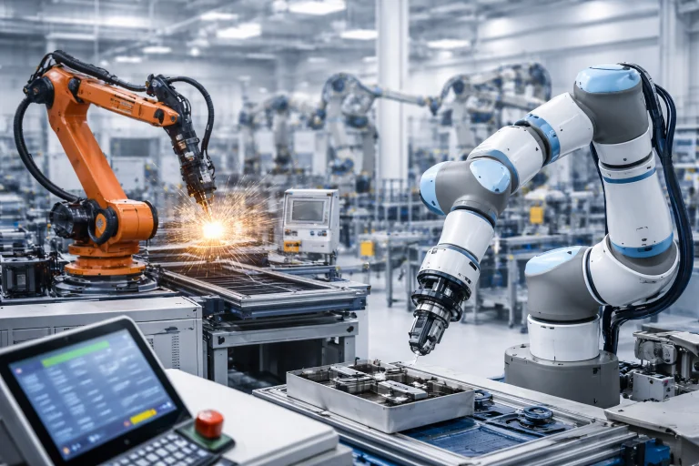
Industrial robotics systems are designed for high-precision, repeatable tasks in structured manufacturing environments such as assembly lines, welding stations, and automated production cells. Traditional industrial robot arms perform fast, powerful operations like welding, machining, and material handling, while collaborative robots (cobots) are engineered to work safely alongside human operators. Together, these systems form integrated automation cells that combine mechanical precision, sensor feedback, and advanced control algorithms to increase production efficiency. Modern industrial robotics is also closely connected with Industry 4.0 technologies, where robots exchange real-time data with digital manufacturing systems to improve productivity, reliability, and quality control.
Interactive Quick Review: Industrial & Cobot Fundamentals
Test your understanding of high-throughput industrial environments and collaborative working spaces before exploring kinematics and dynamics equations:
1. What is the fundamental operational focus of industrial robotics compared to research or field robotics?
Answer: Industrial robotics focuses on high-throughput, micrometer-level repeatability, structural stiffness, and production efficiency in highly structured environments, rather than autonomous mapping or adapting to unstructured outdoor terrain.
2. How do collaborative robots (cobots) differ mechanically and operationally from traditional heavy industrial manipulators?
Answer: Cobots feature lightweight, rounded structures, lower payloads, integrated torque/force sensing, and force-limited actuation, allowing them to share workspaces with humans without physical safety cages under ISO/TS 15066 safety standards.
Glossary of Key Terminology
Key foundational terminology defining industrial manipulators, collaborative robotics, and automated manufacturing:
Architecture of Industrial Manipulators
Most industrial robots are serial manipulators with six degrees of freedom (6-DOF). Degrees of freedom refer to the independent joint motions that allow the robot arm to position and orient its tool — known as the end-effector — anywhere within its reachable workspace.
Let:
- \(\mathbf{q} = [q_1, q_2, \dots, q_6]^T\): vector of joint coordinates describing the robot configuration
- \(\mathbf{T}(\mathbf{q})\): homogeneous transformation matrix (\(4 \times 4\)) describing the position and orientation (pose) of the end-effector relative to the base coordinate frame
The forward kinematics problem computes the pose of the end-effector from the joint coordinates:
$$\mathbf{T}(\mathbf{q}) = \mathbf{T}_1(q_1) \mathbf{T}_2(q_2) \dots \mathbf{T}_6(q_6)$$where each \(\mathbf{T}_i(q_i)\) represents the geometric coordinate transformation contributed by joint \(i\), commonly derived using Denavit–Hartenberg (D-H) parameters. The analytical foundations of this representation are developed in depth in Robot Kinematics and Dynamics.
Industrial manipulators are engineered to maximize mechanical stability, positional precision, and structural rigidity. Key design priorities include:
- Structural rigidity to eliminate deflection under heavy dynamic and cutting loads
- Zero-backlash gearing (harmonic drives or cycloidal reducers) to preserve positioning accuracy
- High-torque-density brushless permanent magnet servomotors for compact, responsive actuation
- Thermal stability and thermal compensation algorithms to prevent geometric expansion errors during continuous production shifts
Dynamic Modeling and Torque Control
Even in structured factory cells, high-speed robotic trajectory execution demands dynamic model inversion. The forces and torques required at the actuator output depend nonlinearly on the configuration, angular velocity, and acceleration of every link.
Let:
- \(\mathbf{q}\): joint position vector
- \(\dot{\mathbf{q}}\): joint velocity vector
- \(\ddot{\mathbf{q}}\): joint acceleration vector
- \(\boldsymbol{\tau}\): vector of actuator torques applied at each joint
The rigid-body equations of motion for an \(n\)-DOF industrial manipulator are formulated via the Euler-Lagrange equations:
$$\mathbf{M}(\mathbf{q})\ddot{\mathbf{q}} + \mathbf{C}(\mathbf{q},\dot{\mathbf{q}})\dot{\mathbf{q}} + \mathbf{G}(\mathbf{q}) = \boldsymbol{\tau}$$where:
- \(\mathbf{M}(\mathbf{q})\): symmetric, positive-definite mass/inertia matrix representing system kinetic energy distribution
- \(\mathbf{C}(\mathbf{q}, \dot{\mathbf{q}})\dot{\mathbf{q}}\): vector of Coriolis and centrifugal torques arising from coupled joint velocities
- \(\mathbf{G}(\mathbf{q})\): configuration-dependent gravity torque vector
In high-speed assembly and seam welding, ignoring coupled dynamics causes trajectory tracking errors, severe joint overshoot, and vibration. Modern industrial controllers implement computed-torque control (feedback linearization) to cancel these nonlinearities:
$$\boldsymbol{\tau} = \mathbf{M}(\mathbf{q})\left(\ddot{\mathbf{q}}_d + \mathbf{K}_v(\dot{\mathbf{q}}_d - \dot{\mathbf{q}}) + \mathbf{K}_p(\mathbf{q}_d - \mathbf{q})\right) + \mathbf{C}(\mathbf{q},\dot{\mathbf{q}})\dot{\mathbf{q}} + \mathbf{G}(\mathbf{q})$$Advanced control architectures are explored further in Advanced Control Systems in Robotics.
Precision, Accuracy, and Repeatability
Industrial manipulators are categorized using repeatability rather than absolute positioning accuracy. Repeatability describes how consistently the manipulator returns to the exact same taught coordinate under identical operating conditions.
Let:
- \(\mathbf{p}_d\): desired end-effector target coordinate
- \(\mathbf{p}_i\): measured physical position attained during trial \(i\)
- \(\Delta \mathbf{p}_i = \mathbf{p}_i - \mathbf{p}_d\): Euclidean positioning error vector during trial \(i\)
- \(\bar{\mathbf{p}}\): barycenter (mean coordinate) of \(N\) experimental runs
According to ISO 9283, positioning repeatability (\(R_p\)) is defined as:
$$R_p = \bar{l} + 3S_l$$where \(\bar{l}\) is the mean distance from the barycenter and \(S_l\) is the sample standard deviation:
$$S_l = \sqrt{\frac{1}{N-1}\sum_{i=1}^N \left( \|\mathbf{p}_i - \bar{\mathbf{p}}\| - \bar{l} \right)^2}$$Standard industrial robots achieve repeatability tolerances on the order of \(\pm 0.01\text{ mm}\) to \(\pm 0.02\text{ mm}\) (\(\pm 10\text{ to }20\text{ }\mu\text{m}\)), whereas absolute positioning accuracy without vision or external metrology calibration is typically around \(\pm 0.5\text{ mm}\) to \(\pm 1.5\text{ mm}\) due to link compliance, kinematic manufacturing tolerances, and thermal expansion.
Automation Cells and Integrated Manufacturing
Industrial robots operate as part of coordinated manufacturing cells consisting of conveyors, machine vision sensors, safety light curtains, pneumatic grippers, and Programmable Logic Controllers (PLCs).
Common industrial tasks include:
- Pick-and-place packaging and flexible bin picking
- Automated spot welding and continuous arc seam welding
- High-precision multi-axis machining, deburring, and routing
- Surface finishing, powder coating, and spray painting
- Micro-electronic assembly and cleanroom silicon wafer handling
A primary economic performance metric in industrial automation is cycle time (\(T_{\text{cycle}}\)), which directly dictates hourly production throughput (\(Q\)):
$$T_{\text{cycle}} = T_{\text{move}} + T_{\text{process}}$$ $$Q = \frac{3600}{T_{\text{cycle}}} \quad \left[\text{units per hour}\right]$$Optimizing trajectories through jerk-bounded S-curve profiling minimizes \(T_{\text{move}}\) without exciting mechanical arm resonances.
Collaborative Robots (Cobots) and Human-Robot Safety
Collaborative robots (cobots) are designed to work alongside human operators in uncaged manufacturing spaces. They adhere to international safety specifications governed by ISO 10218-1/2 and technical specification ISO/TS 15066.
Typical engineering characteristics of cobots include:
- Lower total moving mass and streamlined, rounded casing geometry to prevent pinch and shear points
- Integrated joint torque sensors (strain gauges) and motor current monitoring for rapid collision detection
- Power and force limiting (PFL) architectures that maintain impact energy below biomechanical pain thresholds
- Direct lead-through (hand-guiding) intuitive programming modes for rapid batch changeovers
In collaborative contact scenarios, safety logic requires that transient impact forces and sustained clamping forces satisfy:
$$F_{\text{contact}} \le F_{\text{limit}}$$Cobots frequently implement active compliance control such as impedance or admittance control. An end-effector impedance relationship is governed by:
$$\mathbf{M}_d (\ddot{\mathbf{x}} - \ddot{\mathbf{x}}_d) + \mathbf{B}_d (\dot{\mathbf{x}} - \dot{\mathbf{x}}_d) + \mathbf{K}_d (\mathbf{x} - \mathbf{x}_d) = -\mathbf{F}_{\text{ext}}$$where \(\mathbf{M}_d\), \(\mathbf{B}_d\), and \(\mathbf{K}_d\) represent virtual target mass, damping, and stiffness matrices. By tuning virtual stiffness \(\mathbf{K}_d\) dynamically, the cobot yields softly upon physical contact, limiting impact forces.
Industry 4.0, Digital Twins, and Networked Manufacturing
Modern industrial robots are embedded within networked Cyber-Physical Systems (CPS) under the Industry 4.0 paradigm. Real-time sensory data is continuously harvested across Industrial Ethernet protocols (EtherCAT, PROFINET) and edge computing nodes.
Let:
- \(D(t)\): real-time telemetry stream collected from embedded physical sensors (motor current, joint vibration, bearing temperature)
- \(\hat{D}(t)\): predicted operational data simulated in real time by a physics-based digital twin
- \(r(t) = \|D(t) - \hat{D}(t)\|\): residual error signal used for predictive health monitoring
Under normal operating conditions:
$$D(t) \approx \hat{D}(t) \quad \text{implying} \quad r(t) \le \epsilon_{\text{threshold}}$$When residual \(r(t)\) exceeds calibrated thresholds, the digital twin detects mechanical wear, lubrication degradation, or gearbox backlash long before mechanical failure halts the assembly line. Distributed computing and cloud integration architectures are explored further in Cloud Robotics and Edge Intelligence.
Engineering Challenges & Technical Solutions
Deploying industrial manipulators and cobots involves resolving complex conflicts between structural mechanics, cycle-time efficiency, deterministic communication, and biological safety:
The Challenge: Traditional articulated robots weigh 15 to 30 times their rated payload capacity to prevent flexural deformation during high-speed moves. In collaborative robotics, this large mass generates substantial kinetic energy (\(E_k = \frac{1}{2}mv^2\)) that could cause fatal blunt-force trauma during an uncaged collision.
- Topology Optimization & Carbon Shells: Cobot engineers achieve structural stiffness with minimal moving mass using finite-element-optimized thin-walled cast aluminum alloys and hollow carbon-fiber structural links.
- Inertial Mass Concentration: Actuators, brakes, and harmonic drives are positioned closer to the robot base, routing drive torque through concentric torque tubes or tensioned timing belts to drastically reduce the moving link inertia matrix \(\mathbf{M}(\mathbf{q})\).
The Challenge: Standard spur or planetary gear trains exhibit mechanical backlash (typically 1 to 5 arcminutes), producing positioning errors of several millimeters at an extended 1-meter reach. Conversely, while zero-backlash harmonic drives (strain-wave gears) eliminate backlash, their flexible steel cups (flexsplines) undergo cyclic radial deformation, making them vulnerable to fatigue failure under heavy shock loads.
- Hybrid Gear Architecture: High-ratio (\(50:1\) to \(160:1\)) strain-wave gears paired with cross-roller bearings are deployed in wrist joints to absorb combined radial and axial moments.
- Cycloidal Pin-Wheel Reducers: For heavy-payload base and shoulder axes (joints 1, 2, and 3), multi-tooth engagement cycloidal reducers withstand shock loads up to 500% of nominal rating without tooth shear or loss of zero-backlash positioning.
The Challenge: Continuous operation in non-climate-controlled plant environments causes servomotors and gear friction to heat robot arm links by \(\Delta T = 20^\circ\text{C}\text{ to }35^\circ\text{C}\). For a 1.2-meter steel arm, thermal expansion (\(\Delta L = \alpha L \Delta T\)) causes Tool Center Point (TCP) drift exceeding \(300\text{ }\mu\text{m}\), violating micro-machining and aerospace drilling tolerances.
- Real-Time Kinematic Thermal Compensation: Embedded multi-point PT100 temperature sensors monitor heat profiles along each link, allowing the controller to dynamically update kinematic link length parameters in the transformation matrices \(\mathbf{T}_i(q_i)\).
- Closed-Loop Optical Recalibration: The manipulator executes periodic automated calibration routines by touching an optical probe to a calibrated reference sphere, resetting Cartesian tool offsets without interrupting production schedules.
The Challenge: Cobot safety limits under ISO/TS 15066 enforce strict biomechanical thresholds for human contact (e.g., maximum \(140\text{ N}\) force and \(0.49\text{ J}\) transient energy for the chest and arm). If controller communication suffers from packet jitter or slow cycle times, contact forces can spike to dangerous levels before the brakes engage.
- Dual-Channel Joint Encoders & Torque Hubs: Collaborative joints integrate dual high-resolution encoders (pre- and post-gearbox) alongside dedicated strain-gauge torque sensors inside joint output hubs.
- Deterministic Sub-Millisecond Fieldbuses: Sensory telemetries stream over EtherCAT or SERCOS III buses cycling at \(1\text{ to }4\text{ kHz}\) (\(\le 1\text{ ms}\) cycle time), allowing dual-core FPGA safety watchdogs to trigger Safe Torque Off (STO) and mechanical brake clamping within \(3\text{ to }5\text{ ms}\) of impact detection.
The Challenge: In 6-DOF industrial manipulators, when the wrist center lines up with the arm's base axis (wrist singularity) or the forearm and upper arm align (elbow singularity), the kinematic Jacobian matrix \(\mathbf{J}(\mathbf{q})\) loses full rank. Inverting the Jacobian to maintain constant Cartesian end-effector velocity (\(\Delta \dot{\mathbf{q}} = \mathbf{J}^{-1} \Delta \dot{\mathbf{x}}\)) demands mathematically infinite joint velocities, tripping servo overspeed protections.
- Yoshikawa Manipulability Tracking: Advanced trajectory generators continuously monitor the manipulability index: $$w(\mathbf{q}) = \sqrt{\det\left(\mathbf{J}(\mathbf{q})\mathbf{J}(\mathbf{q})^T\right)}$$
- Damped Least-Squares (Levenberg-Marquardt) Inversion: As the arm approaches a singularity (\(w(\mathbf{q}) \to 0\)), the controller smoothly transitions from pure Jacobian inversion to regularized damping: $$\mathbf{J}^*(\mathbf{q}) = \mathbf{J}^T \left( \mathbf{J} \mathbf{J}^T + \lambda^2 \mathbf{I} \right)^{-1}$$ where \(\lambda\) is a dynamic damping factor, bounding joint velocities within safe motor capabilities at the cost of imperceptible Cartesian deviations.
🎯 Career Guidance Tool Is Industrial Robotics & Smart Manufacturing Right For You?Explore industrial robotics integration, cobot applications, digital twin modeling, and advanced automation engineering career pathways. | Explore Career Options → |
Interactive Quick Review: Dynamics, Repeatability & Digital Twins
Reinforce key concepts regarding dynamic torque compensation, repeatability standards, and digital twin monitoring before reviewing the FAQ:
1. Why do industrial robots specify repeatability (\(R_p\)) rather than absolute positioning accuracy as their primary benchmark?
Answer: Industrial manufacturing processes (such as spot welding or pick-and-place) rely on returning to programmed coordinates thousands of times with micrometer consistency (\(\pm 0.02\text{ mm}\)), which repeatability measures directly. Systematic absolute accuracy offsets can be calibrated out via taught waypoints.
2. How does a digital twin simulation identify mechanical degradation or wear in an Industry 4.0 robot?
Answer: By continuously evaluating the residual difference \(r(t) = \|D(t) - \hat{D}(t)\|\) between real-time sensor telemetries (current, vibration, temperature) and the physics simulation; sustained residual deviations indicate friction build-up, backlash, or bearing wear.
External References and Further Reading
To explore authoritative engineering standards, manufacturing statistics, and industrial automation research, consult the following sources:
- International Federation of Robotics (IFR) – Provides global industrial robotics adoption statistics, operational stock data, and annual manufacturing reports.
- ISO 10218-1: Robots and Robotic Devices — Safety Requirements – The primary international standard specifying safety design and integration guidelines for industrial manipulators.
- ISO/TS 15066: Collaborative Robots – Technical specification establishing quantitative biomechanical thresholds for speed, separation monitoring, and power-and-force-limited contact.
- Association for Advancing Automation (A3) – Global trade association delivering robotics technical specifications, safety training, and North American industrial adoption metrics.
Frequently Asked Questions about Industrial Robotics Systems and Cobots
What is the primary operational difference between a traditional industrial robot and a cobot?
Traditional industrial robots are heavy, rigid machines optimized for maximum speed and payload within barricaded work cells protected by safety fences and interlock curtains. Cobots are lightweight, speed- and force-limited arms engineered with rounded profiles and integrated torque sensors, enabling them to share open workstations alongside human operators under ISO/TS 15066 standards.
Why are 6 degrees of freedom (6-DOF) considered standard for industrial articulated arms?
Six degrees of freedom (three translational axes \(x, y, z\) and three rotational orientations roll, pitch, yaw) represent the minimum mathematical requirement to place an end-effector tool at any arbitrary pose within a 3D workspace. Additional joints (\(7+\text{ DOF}\)) create kinematic redundancy used for obstacle avoidance.
How does model-based torque control compensate for high-speed dynamic forces?
Model-based control continuously solves the dynamic equation \(\boldsymbol{\tau} = \mathbf{M}(\mathbf{q})\ddot{\mathbf{q}} + \mathbf{C}(\mathbf{q}, \dot{\mathbf{q}})\dot{\mathbf{q}} + \mathbf{G}(\mathbf{q})\) in real time. By calculating the exact inertial, Coriolis, centrifugal, and gravitational forces acting on each link, the controller feeds forward the required motor currents, eliminating servo lag and trajectory tracking errors.
What is the difference between repeatability and absolute accuracy?
Repeatability measures the robot's ability to return to the exact same physical coordinate over thousands of cycles (typically \(\pm 0.01\text{ to }\pm 0.02\text{ mm}\)). Absolute accuracy measures the robot's ability to hit a coordinate commanded directly from theoretical CAD space without taught adjustments (typically \(\pm 0.5\text{ to }\pm 1.5\text{ mm}\) due to link compliance and machining tolerances).
End-of-Page Exercises: Review, Thought-Provoking & Engineering Problems
Section 1: Foundational Review Questions & Answers
1. What geometric transformation matrix maps a 6-DOF robot's joint angles to its end-effector pose?
Answer: The forward kinematics homogeneous transformation matrix \(\mathbf{T}(\mathbf{q}) = \mathbf{T}_1(q_1) \mathbf{T}_2(q_2) \dots \mathbf{T}_6(q_6)\).
2. In the dynamic equation \(\mathbf{M}(\mathbf{q})\ddot{\mathbf{q}} + \mathbf{C}(\mathbf{q}, \dot{\mathbf{q}})\dot{\mathbf{q}} + \mathbf{G}(\mathbf{q}) = \boldsymbol{\tau}\), what physical phenomenon does \(\mathbf{C}(\mathbf{q}, \dot{\mathbf{q}})\) represent?
Answer: Velocity-dependent Coriolis and centrifugal forces generated by coupled link motions.
3. What mathematical formula defines positioning repeatability (\(\sigma\)) across \(N\) experimental trials?
Answer: \(\sigma = \sqrt{\frac{1}{N} \sum_{i=1}^N \|\Delta \mathbf{p}_i\|^2}\), where \(\Delta \mathbf{p}_i\) is the error vector between trial position and commanded target position.
4. How is total automation cell cycle time (\(T_{\text{cycle}}\)) calculated?
Answer: By summing motion transfer duration and process execution duration: \(T_{\text{cycle}} = T_{\text{move}} + T_{\text{process}}\).
5. What safety condition governs contact force enforcement in collaborative robots?
Answer: Measured contact force must remain below or equal to the allowable biomechanical threshold: \(F_{\text{contact}} \le F_{\text{limit}}\).
6. In spring impedance control \(F = K(x_d - x)\), what does parameter \(K\) represent?
Answer: The virtual stiffness constant of the end-effector controller, dictating reactive force per unit displacement.
7. What mathematical relationship describes digital twin signal convergence in Industry 4.0?
Answer: Real-time physical sensor telemetry matches predicted virtual simulation outputs: \(D(t) \approx \hat{D}(t)\).
8. What mechanical design property minimizes elastic link deflection during heavy milling or machining tasks?
Answer: High structural flexural rigidity achieved through thick-walled cast steel or alloy construction and widely spaced preloaded bearings.
9. What mechanical gear mechanism eliminates backlash from industrial manipulator joints?
Answer: Zero-backlash harmonic drive (strain wave) gearsets and high-precision cycloidal pin-wheel reducers.
10. List four primary manufacturing operations executed by industrial articulated arms.
Answer: High-speed pick-and-place packaging, spot and continuous arc welding, precision adhesive dispensing, and robotic surface machining.
Section 2: Analytical & Thought-Provoking Questions
1. Why can a robot with excellent repeatability (\(\pm 0.01\text{ mm}\)) exhibit mediocre absolute positioning accuracy (\(\pm 1.5\text{ mm}\))?
Answer: Repeatability measures statistical dispersion around an arbitrary arrived point. Unmodeled link elastic deflection, thermal expansion, gearbox backlash, joint encoder zero-point offsets, and machining tolerances introduce systematic coordinate shifts between CAD models and physical space, impairing absolute accuracy while preserving tight repeatability.
2. How does high-speed motion in heavy manipulators create trade-offs between cycle time and mechanical lifespan?
Answer: Maximizing joint acceleration reduces move time \(T_{\text{move}}\), improving production throughput. However, rapid acceleration elevates peak dynamic inertial torques (\(\mathbf{M}(\mathbf{q})\ddot{\mathbf{q}}\)), accelerating gear tooth pitting, fatigue wear in bearings, and thermal stress on motor windings.
3. Why are collaborative robots currently unsuitable for heavy high-speed tasks like automotive hot stamping?
Answer: Cobot safety standards (ISO/TS 15066) mandate strict limits on kinetic transfer energy (\(E = \frac{1}{2}mv^2\)) and impact forces. Heavy payloads manipulated at high process speeds carry kinetic energy levels that would cause fatal blunt-force trauma upon human impact, making uncaged cobot operation physically impossible under current safety regulations.
4. How do thermal fluctuations over a 24-hour manufacturing shift degrade sub-millimeter precision?
Answer: Ambient temperature swings and internal motor heat cause linear expansion of metal links (\(\Delta L = \alpha L \Delta T\)). For a steel arm with \(L = 1.0\text{ m}\), a \(20^\circ\text{C}\) temperature rise produces \(240\text{ }\mu\text{m}\) of positional drift, exceeding micrometer assembly tolerances unless compensated via thermal modeling.
5. How does admittance control differ conceptually from impedance control?
Answer: Impedance control accepts motion deviation as input and outputs a restoration force (behaving like a software spring). Admittance control measures external applied force (via a wrist 6-axis force/torque sensor) and outputs a corresponding velocity/position trajectory, enabling stiff, heavy manipulators to be effortlessly hand-guided.
6. Why is kinematic singularity avoidance essential in trajectory planning for 6-DOF industrial arms?
Answer: At kinematic singularities, the manipulator Jacobian matrix loses full rank (\(\det(\mathbf{J}) = 0\)). Inverting the Jacobian to maintain constant Cartesian end-effector speed requires infinite joint velocity (\(\dot{\mathbf{q}} = \mathbf{J}^{-1} \dot{\mathbf{x}}\)), causing actuator saturation, severe controller instability, and automatic emergency trip stops.
7. How does edge computing reduce network bandwidth in smart Industry 4.0 factories?
Answer: Local edge gateways run high-frequency FFT vibration analysis and anomaly detection right at the machine cell, transmitting only extracted feature vectors and health indicators (\(D(t)\)) to enterprise clouds rather than multi-gigabyte raw sensor waveform streams.
8. What cybersecurity risks emerge when interconnecting robot cells to enterprise IT networks?
Answer: Bridging OT factory networks to IT enterprise networks creates attack vectors for unauthorized remote access, firmware corruption, and malicious trajectory injection that could override software safety zones, causing physical damage or human injury.
9. How does 3D depth-vision guidance improve automated bin picking over fixed mechanical fixtures?
Answer: Fixed fixtures require mechanical bowl feeders to orient parts rigidly. 3D point cloud segmentation identifies randomly oriented, jumbled components directly within bulk bins, calculates 6-DOF grasp poses, and generates collision-free extraction paths on the fly.
10. How does gravity feedforward compensation \(\mathbf{G}(\mathbf{q})\) optimize motor sizing in articulated manipulators?
Answer: By computing the exact static gravitational holding torque analytically for any arm configuration, controllers supply the required feedforward holding currents directly. This prevents feedback integrator lag, eliminates steady-state droop, reduces thermal buildup, and allows smaller servomotors to be specified.
11. Why is lead-through manual teaching advantageous for high-mix, low-volume manufacturing?
Answer: High-mix production requires frequent reprogramming. Lead-through teaching allows floor technicians to physically guide the cobot arm through desired waypoints without writing robot code, cutting batch changeover times from days to minutes.
12. How does mounting an articulated robot on an inverted ceiling rail affect dynamic modeling?
Answer: Ceiling mounting inverts the gravity vector orientation relative to the robot base frame (\(\mathbf{g} = [0, 0, +9.81]^T\text{ m/s}^2\)). The controller's internal gravity vector matrix \(\mathbf{G}(\mathbf{q})\) must be updated, or feedforward torques will act in the direction of gravity rather than opposing it, causing severe arm collapse.
Section 3: Numerical Engineering Problems & Solutions
A precision industrial robot returns to a taught target assembly coordinate across \(N = 5\) test trials. The measured Euclidean positioning error distances \(\|\Delta \mathbf{p}_i\|\) are: \(0.012\text{ mm}\), \(0.018\text{ mm}\), \(0.015\text{ mm}\), \(0.022\text{ mm}\), and \(0.013\text{ mm}\). Calculate the robot repeatability standard deviation (\(\sigma\)) in millimeters.
1. Square each error distance: $$(0.012)^2 = 0.000144\text{ mm}^2, \quad (0.018)^2 = 0.000324\text{ mm}^2, \quad (0.015)^2 = 0.000225\text{ mm}^2$$ $$(0.022)^2 = 0.000484\text{ mm}^2, \quad (0.013)^2 = 0.000169\text{ mm}^2$$ 2. Sum squared errors: $$\sum \|\Delta \mathbf{p}_i\|^2 = 0.000144 + 0.000324 + 0.000225 + 0.000484 + 0.000169 = 0.001346\text{ mm}^2$$ 3. Divide by sample count \(N = 5\): $$\text{MSE} = \frac{0.001346}{5} = 0.0002692\text{ mm}^2$$ 4. Take the square root: $$\sigma = \sqrt{0.0002692} \approx 0.0164\text{ mm}$$ Final Answer: Robot positioning repeatability is approximately \(\pm 0.0164\text{ mm}\) (\(16.4\text{ }\mu\text{m}\)).
An automated robotic spot-welding cell performs 12 weld spots on an automotive chassis. Transfer movement between weld spots takes a total move time of \(T_{\text{move}} = 14.5\text{ s}\), while welding execution takes \(T_{\text{process}} = 9.5\text{ s}\). Calculate the total cycle time per chassis (\(T_{\text{cycle}}\)) in seconds, and determine the maximum hourly production throughput (\(Q\)) in chassis units per hour.
1. Calculate total cycle time: $$T_{\text{cycle}} = T_{\text{move}} + T_{\text{process}} = 14.5\text{ s} + 9.5\text{ s} = 24.0\text{ seconds}$$ 2. Compute hourly throughput: $$Q = \frac{3600\text{ seconds/hour}}{24.0\text{ seconds/chassis}} = 150\text{ chassis/hour}$$ Final Answer: Total cycle time is \(24.0\text{ seconds}\), yielding an hourly production throughput of \(150\text{ chassis per hour}\).
A collaborative robot arm equipped with joint torque sensors measures a transient contact force of \(F_{\text{contact}} = 115\text{ N}\) when contacting an operator's forearm. If ISO/TS 15066 safety guidelines establish a maximum allowable force limit of \(F_{\text{limit}} = 140\text{ N}\) for forearm contact, verify whether the safety condition \(F_{\text{contact}} \le F_{\text{limit}}\) is satisfied and calculate the force safety margin.
1. Evaluate safety condition: $$115\text{ N} \le 140\text{ N} \Rightarrow \text{Condition is satisfied}$$ 2. Calculate force safety margin: $$\text{Margin} = F_{\text{limit}} - F_{\text{contact}} = 140\text{ N} - 115\text{ N} = 25\text{ N}$$ Final Answer: The safety condition is satisfied with a force margin of \(25\text{ N}\).
A cobot end-effector utilizes an impedance safety controller modeled as \(F = K(x_d - x)\). The virtual stiffness is set to \(K = 350\text{ N/m}\). During accidental contact with a workpiece, the end-effector is displaced from its target position by \((x_d - x) = 0.08\text{ m}\). Calculate the resulting interaction force \(F\) generated by the virtual impedance controller.
1. Impedance force formula: $$F = K \cdot \Delta x$$ 2. Substitute parameters: $$F = 350\text{ N/m} \times 0.08\text{ m} = 28.0\text{ N}$$ Final Answer: The generated interaction force is \(28.0\text{ N}\).
At a specific trajectory instant, a single rotational joint of an industrial manipulator has link inertia \(M(q) = 2.5\text{ kg}\cdot\text{m}^2\), desired angular acceleration \(\ddot{q} = 4.0\text{ rad/s}^2\), Coriolis/centrifugal torque term \(C(q, \dot{q})\dot{q} = 1.8\text{ N}\cdot\text{m}\), and gravity torque \(G(q) = 12.2\text{ N}\cdot\text{m}\). Calculate the total required actuator joint torque \(\tau\) using the equation \(\tau = M(q)\ddot{q} + C(q, \dot{q})\dot{q} + G(q)\).
1. Calculate inertial torque component: $$\tau_{\text{inertial}} = M(q)\ddot{q} = 2.5\text{ kg}\cdot\text{m}^2 \times 4.0\text{ rad/s}^2 = 10.0\text{ N}\cdot\text{m}$$ 2. Sum dynamic torque components: $$\tau = 10.0\text{ N}\cdot\text{m} + 1.8\text{ N}\cdot\text{m} + 12.2\text{ N}\cdot\text{m} = 24.0\text{ N}\cdot\text{m}$$ Final Answer: Total required actuator joint torque is \(24.0\text{ N}\cdot\text{m}\).
A digital twin diagnostics framework monitors an industrial joint motor current. The real-time physical sensor data stream records peak current \(D(t) = 18.4\text{ A}\), while the virtual simulation predicts \(\hat{D}(t) = 16.0\text{ A}\). Calculate the absolute residual error \(|D(t) - \hat{D}(t)|\) and the percentage deviation relative to the predicted value.
1. Absolute residual error: $$r(t) = |18.4\text{ A} - 16.0\text{ A}| = 2.4\text{ A}$$ 2. Percentage deviation relative to prediction: $$\text{Error} = \left(\frac{2.4}{16.0}\right) \times 100\% = 15.0\%$$ Final Answer: Absolute error is \(2.4\text{ A}\), representing a \(15.0\%\) deviation (indicating mechanical friction build-up).
A lightweight cobot arm component with effective moving mass \(m = 6.0\text{ kg}\) moves at speed \(v_1 = 1.2\text{ m/s}\). Calculate its kinetic energy \(E_1\). If speed is reduced to \(v_2 = 0.6\text{ m/s}\) upon detecting human proximity, calculate the new kinetic energy \(E_2\) and state the reduction ratio.
1. Initial kinetic energy: $$E_1 = \frac{1}{2} m v_1^2 = 0.5 \times 6.0\text{ kg} \times (1.2\text{ m/s})^2 = 3.0 \times 1.44 = 4.32\text{ J}$$ 2. Reduced kinetic energy: $$E_2 = \frac{1}{2} m v_2^2 = 0.5 \times 6.0\text{ kg} \times (0.6\text{ m/s})^2 = 3.0 \times 0.36 = 1.08\text{ J}$$ 3. Ratio check: $$\frac{E_1}{E_2} = \frac{4.32}{1.08} = 4.0$$ Final Answer: Initial energy is \(4.32\text{ J}\); halving speed reduces kinetic energy to \(1.08\text{ J}\) (a 4-fold kinetic energy reduction).
Upgrading an assembly cell from manual labor to a 6-DOF industrial robot arm reduces movement time between components from \(T_{\text{move, manual}} = 18.0\text{ s}\) to \(T_{\text{move, robot}} = 4.5\text{ s}\), with process execution constant at \(T_{\text{process}} = 5.5\text{ s}\). Calculate manual cycle time, robotic cycle time, and net cycle time savings per assembly.
1. Manual cycle time: $$T_{\text{manual}} = 18.0\text{ s} + 5.5\text{ s} = 23.5\text{ seconds}$$ 2. Robotic cycle time: $$T_{\text{robot}} = 4.5\text{ s} + 5.5\text{ s} = 10.0\text{ seconds}$$ 3. Time savings per unit: $$\Delta T = 23.5\text{ s} - 10.0\text{ s} = 13.5\text{ seconds}$$ Final Answer: Deployment reduces cycle time from \(23.5\text{ s}\) to \(10.0\text{ s}\), saving \(13.5\text{ seconds per assembly}\).
A steel manipulator link has an initial nominal length \(L = 0.8\text{ m}\) at \(20^\circ\text{C}\). Continuous high-speed operation elevates link temperature to \(45^\circ\text{C}\) (\(\Delta T = 25\text{ K}\)). Given a linear thermal expansion coefficient for steel of \(\alpha = 12 \times 10^{-6}\text{ K}^{-1}\), calculate the physical length expansion \(\Delta L\) in micrometers (\(\mu\text{m}\)).
1. Thermal expansion formula: $$\Delta L = \alpha \cdot L \cdot \Delta T$$ 2. Substitute numerical values: $$\Delta L = (12 \times 10^{-6}\text{ K}^{-1}) \times 0.8\text{ m} \times 25\text{ K} = 2.4 \times 10^{-4}\text{ m}$$ 3. Convert to micrometers: $$2.4 \times 10^{-4}\text{ m} \times 10^6\text{ }\mu\text{m/m} = 240\text{ }\mu\text{m}\text{ (0.24 mm)}$$ Final Answer: Thermal expansion increases link length by \(240\text{ }\mu\text{m}\) (\(0.24\text{ mm}\)).
An industrial joint motor produces high-speed input torque \(\tau_{\text{in}} = 0.45\text{ N}\cdot\text{m}\). It drives a zero-backlash harmonic drive with gear reduction ratio \(N_{\text{gear}} = 100:1\) and mechanical efficiency \(\eta = 85\%\) (\(0.85\)). Calculate the output torque \(\tau_{\text{out}}\) delivered to the arm link.
1. Output torque formula: $$\tau_{\text{out}} = \tau_{\text{in}} \times N_{\text{gear}} \times \eta$$ 2. Substitute values: $$\tau_{\text{out}} = 0.45\text{ N}\cdot\text{m} \times 100 \times 0.85 = 38.25\text{ N}\cdot\text{m}$$ Final Answer: Joint output torque delivered to the link is \(38.25\text{ N}\cdot\text{m}\).
A 3D depth camera locates a component for robotic bin picking. The algorithm computes Cartesian point cloud registration errors across coordinate axes of \(\Delta x = 0.03\text{ mm}\), \(\Delta y = -0.04\text{ mm}\), and \(\Delta z = 0.00\text{ mm}\) relative to the CAD model origin. Calculate the Euclidean 3D positioning error magnitude \(\|\Delta \mathbf{p}\|\) in millimeters.
1. Euclidean magnitude formula: $$\|\Delta \mathbf{p}\| = \sqrt{(\Delta x)^2 + (\Delta y)^2 + (\Delta z)^2}$$ 2. Square coordinate components: $$(0.03)^2 = 0.0009, \quad (-0.04)^2 = 0.0016, \quad (0.00)^2 = 0$$ 3. Sum and square root: $$\|\Delta \mathbf{p}\| = \sqrt{0.0009 + 0.0016} = \sqrt{0.0025} = 0.05\text{ mm}$$ Final Answer: Euclidean registration error magnitude is \(0.05\text{ mm}\) (\(50\text{ }\mu\text{m}\)).
A cobot model has a maximum rated safety payload capacity of \(M_{\text{max}} = 10.0\text{ kg}\). The end-effector pneumatic tool weighs \(M_{\text{tool}} = 2.3\text{ kg}\), and it grasps an engine casting weighing \(M_{\text{part}} = 6.8\text{ kg}\). Calculate the total combined payload mass carried by the wrist and determine the remaining allowable safety margin.
1. Calculate total payload mass: $$M_{\text{total}} = M_{\text{tool}} + M_{\text{part}} = 2.3\text{ kg} + 6.8\text{ kg} = 9.1\text{ kg}$$ 2. Compare against rated limit: $$9.1\text{ kg} \le 10.0\text{ kg} \Rightarrow \text{Safety limit satisfied}$$ 3. Calculate payload margin: $$\text{Margin} = M_{\text{max}} - M_{\text{total}} = 10.0\text{ kg} - 9.1\text{ kg} = 0.9\text{ kg}$$ Final Answer: Total wrist payload is \(9.1\text{ kg}\), leaving an allowable margin of \(0.9\text{ kg}\).
Industrial Robotics Systems and Cobots — Summary & Wrap-Up
Industrial robotics and collaborative cobots form the operational foundation of modern automated manufacturing. By uniting 6-DOF manipulator kinematics, model-based dynamic torque feedforward, micrometer-level repeatability (\(R_p\)), integrated cell PLCs, compliant impedance safety loops, and Industry 4.0 digital twins, automation engineers build highly productive, flexible, and safe production environments capable of powering modern smart factories.
Interdisciplinary Connections Across Robotics Domains
Industrial robotics principles directly underpin many other specialized fields of robotics. The high-stiffness joint designs and multi-axis kinematic control developed for industrial arms provide the core engineering foundation for precision interventions in Medical and Surgical Robotics. Furthermore, collaborative force-limiting techniques and compliant impedance control are essential across commercial and domestic environments in Service Robotics.
In logistics and supply-chain infrastructure, fixed industrial manipulators work in direct coordination with mobile platforms, as examined in Warehouse Logistics and Autonomous Mobile Robots (AMRs). The vision-guided picking algorithms used in manufacturing cells also adapt to outdoor harvesting environments in Agricultural Robotics.
Mobility technologies represent another important robotics domain. Autonomous vehicles navigating roads are introduced in Autonomous Ground Vehicles, while aerial platforms used for mapping, monitoring, and inspection are discussed in Aerial Robotics and UAV Systems.
Students interested in exploring the foundational mathematics, perception algorithms, and control theory uniting all robotic systems can explore the comprehensive Robotics Hub.