Prepare for University Studies & Career Advancement
Magnetic Dipoles and Materials
Magnetic dipoles and materials explain why some objects respond weakly to magnetic fields, while others become strongly magnetised or even remain magnetic after the external field is removed. This page connects the microscopic idea of magnetic moments with the visible behaviour of materials such as iron, nickel, cobalt, ferrites, permanent magnets, transformer cores, sensors, and magnetic storage systems.
In earlier magnetostatics pages, magnetic fields were produced by steady currents in wires, loops, solenoids, and toroids. This page moves one step deeper. It asks how matter itself responds to magnetic fields. Inside many materials, electrons have magnetic moments. These tiny magnetic dipoles may cancel, align weakly, align strongly, form domains, or resist alignment depending on the material structure.
For students preparing for university physics or engineering, magnetic dipoles and materials form a bridge between basic magnetism and real magnetic technology. The topic explains why some materials are useful for electromagnets, why some make strong permanent magnets, why some are weakly repelled by magnets, and why magnetic behaviour depends on both microscopic structure and macroscopic field conditions.
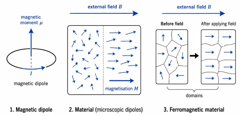
A material’s magnetic behaviour depends on how microscopic magnetic dipoles respond to an external magnetic field and how magnetic domains become aligned.
This illustration introduces magnetic dipoles and magnetic materials using three textbook-style panels. The first panel shows a current loop acting as a magnetic dipole with magnetic moment μ. The second panel shows microscopic dipoles inside a material: some are randomly oriented, while others become partially aligned under an external magnetic field B, producing magnetisation M. The third panel shows ferromagnetic domains before and after a field is applied, helping students see how domain alignment can produce strong magnetisation in magnetic materials.
Learning Pathway
This page belongs to the Magnetostatics cluster under Electricity and Magnetism. It follows the Biot–Savart law and Ampère’s law by showing how matter responds to magnetic fields through magnetic dipoles, magnetisation, domains, and material properties.
Use magnetic circulation and symmetry to calculate magnetic fields around highly regular current distributions.
Magnetic Dipoles and Materials
Explore magnetic moments, dipoles, domains, magnetisation, and how matter responds to magnetic fields.
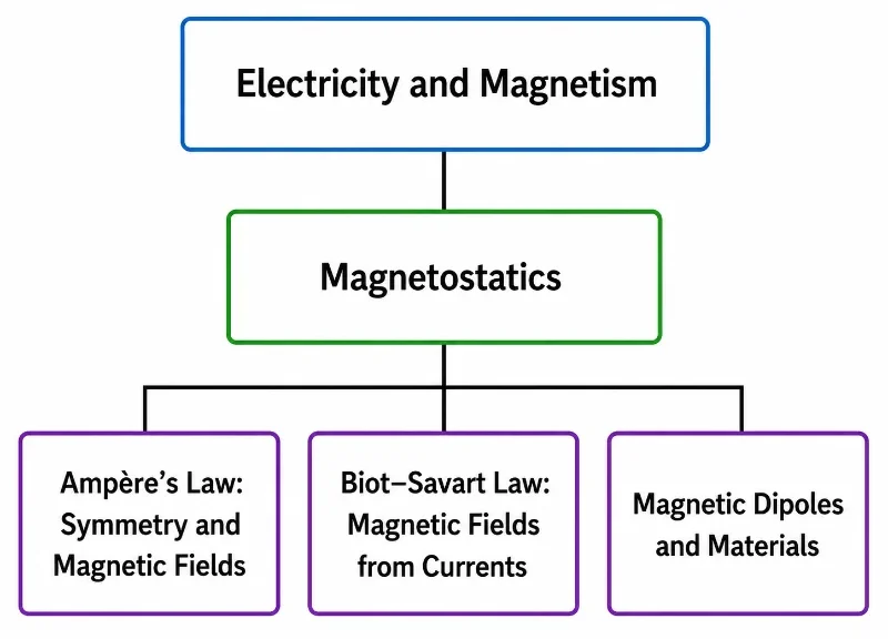
This hierarchy chart shows Magnetostatics within Electricity and Magnetism, with the three child pages rearranged to place Ampère’s Law first, followed by the Biot–Savart Law and Magnetic Dipoles and Materials.
This simple tree chart presents the Magnetostatics cluster within the wider Electricity and Magnetism section of Prep4Uni.online. Electricity and Magnetism appears as the parent area, followed by Magnetostatics as the hub page. The three level-three child pages are shown in a reordered sequence: Ampère’s Law: Symmetry and Magnetic Fields, Biot–Savart Law: Magnetic Fields from Currents, and Magnetic Dipoles and Materials. The chart helps students see that Magnetostatics connects symmetry-based magnetic-field calculation, magnetic fields produced by currents, and the behaviour of magnetic dipoles and materials.
What Magnetic Dipoles and Materials Really Mean
A magnetic dipole is a small magnetic system with a north-like side and a south-like side. A simple model is a tiny current loop: current circulates around a small area, producing a magnetic field similar to that of a small bar magnet. At the microscopic level, electrons in atoms also contribute magnetic moments through their orbital motion and intrinsic spin.
A magnetic material is not magnetic merely because it contains atoms. What matters is how the magnetic moments inside the material combine. In some materials, microscopic magnetic moments cancel almost completely. In others, a small applied field can produce weak alignment. In ferromagnetic materials, groups of magnetic moments can align strongly in domains, producing large magnetic effects.
This makes magnetism in materials both subtle and practical. The same basic idea of magnetic dipoles helps explain weak magnetic response, strong permanent magnets, electromagnets, transformer cores, magnetic sensors, hard drives, speakers, motors, and many scientific instruments.
The Magnetic Dipole Moment
For a small current loop, the magnetic dipole moment is defined by the following vector formulation:
$$\boldsymbol{\mu} = I A \hat{\mathbf{n}}$$
Here, I is the current in the loop, A is the area of the loop, and n̂ is a unit vector perpendicular to the plane of the loop. The direction of μ is found using the right-hand rule: curl the fingers of your right hand in the direction of conventional current, and your thumb points in the direction of the magnetic moment.
For a coil with N identical turns, the collective magnetic dipole moment expression becomes:
$$\boldsymbol{\mu} = N I A \hat{\mathbf{n}}$$
This explains why coils can produce much stronger magnetic effects than a single loop. Each turn contributes a magnetic moment in the same direction, allowing macro-scale reinforcement.
Reading the Magnetic Dipole Moment
To easily utilize the formula across engineering problems, the parameter components are broken down below:
Loop Current (I)
The current in the loop. A larger current produces a linearly larger magnetic dipole moment.
Enclosed Area (A)
The area enclosed by the current loop. A larger loop area expands the spatial range of the dipole moment.
Turn Count (N)
The number of turns in a coil. Stacking more turns multiplies the total constructive magnetic moment output.
Normal Vector (n̂)
The unit vector pointing perpendicular to the loop plane, established via right-hand parameters.
Dipole Moment (μ)
The net magnetic dipole moment vector, measuring both the directional heading and strength of the magnetic system.
The Right-Hand Rule
Curl fingers with conventional current vector directions; the extended thumb gives the vector direction of μ.
Vector Torque and Mechanical Alignment
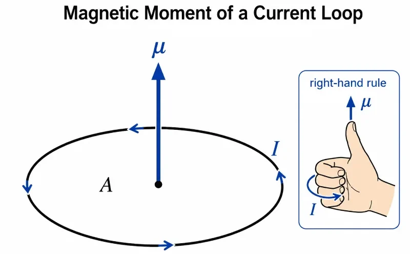
A current loop behaves like a magnetic dipole, with magnetic moment μ pointing perpendicular to the loop according to the right-hand rule.
This diagram shows how a circular current loop produces a magnetic dipole moment. The current I flows around the loop, enclosing an area A. Using the right-hand rule, the curled fingers follow the direction of conventional current, while the thumb points in the direction of the magnetic moment μ. The illustration helps students understand why a current loop can be treated as a small magnetic dipole and how the direction of its magnetic moment is determined.
When a magnetic dipole is placed inside an external magnetic field, it experiences a rotational torque tending to force its magnetic moment vector into parallel alignment with the external field lines. This is modeled by the vector cross-product:
The scalar magnitude of this torque expression expands to:
$$\tau = \mu B \sin\theta$$
Here, θ is the angle between the magnetic moment μ and the magnetic field vector B. The turning torque reaches its absolute maximum when the dipole axis sits perpendicular to the field lines (sin(90°) = 1) and drops to zero when it aligns perfectly parallel or anti-parallel.
Potential Energy of a Magnetic Dipole
A magnetic dipole inside an external field also possesses magnetostatic scalar potential energy:
$$U = -\boldsymbol{\mu}\cdot\mathbf{B}$$
The negative sign inside the scalar dot product proves that the system’s potential energy is minimized when μ points in the exact same direction as B, since cos(0°) = 1 yields U = -μB. This thermodynamic minimization is why atomic dipoles naturally align with applied fields. This behavior underpins compass needles, localized magnetic domains, nuclear magnetic resonance, and shielding technology.
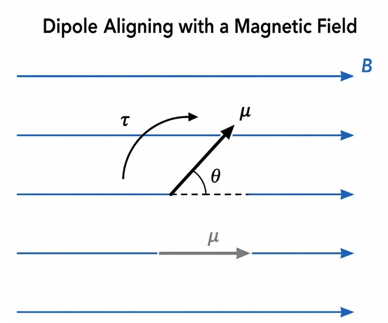
A magnetic dipole in a uniform magnetic field experiences a torque that tends to rotate its magnetic moment into alignment with the field.
This diagram shows how a magnetic dipole behaves in a uniform magnetic field. The magnetic field B points horizontally, while the dipole moment μ is initially at an angle θ to the field. The curved arrow labelled τ represents the torque that turns the dipole toward alignment. A faded aligned position is also shown to indicate the final lower-energy orientation. The picture helps students understand that a magnetic dipole in a uniform field tends to rotate rather than simply move sideways.
The Magnetisation Vector Field
Magnetisation describes the net macroscopic dipole moment density per unit volume inside a material continuum:
If the microscopic atomic moments are randomly oriented due to thermal fluctuations, their vector sum cancels out, making M = 0. When an external field is applied, these moments align, creating a non-zero magnetisation field vector. This parameter bridges the gap between microscopic atomic spins and macroscopic material boundaries.
In real media, the total magnetic flux density B is a collective function of both the external free currents and the internal material response, linked by the constitutive relation:
$$\mathbf{B} = \mu_0(\mathbf{H} + \mathbf{M})$$
Where B is the magnetic flux density, H is the auxiliary magnetic intensity vector driven exclusively by free currents, and M is the magnetisation vector. The total field inside matter is heavily determined by how the material’s internal dipoles react to external stimuli.
Evolution of Material Magnetism: History, Challenges, and Frontiers
To understand how materials interact with steady-state fields, we must examine their historical timeline, engineering core limitations, and future technological frontiers.
Historical Epochs: From Curie’s Law to Weiss Domain Formulations
While ancient civilizations observed natural lodestones, the quantitative formalization of magnetism in matter did not begin until the late 19th century. In 1895, French physicist Pierre Curie discovered that the magnetic susceptibility of paramagnetic materials is inversely proportional to absolute temperature, proving that thermal agitation actively disrupts dipole alignment. In 1906, Pierre Weiss advanced material theory by proposing that ferromagnetic materials contain internal localized magnetic zones, which he termed magnetic domains. He hypothesized that atomic moments within each domain are aligned by a powerful internal field, even in the absence of an external magnetic source. This conceptual framework was later verified by quantum mechanics, which revealed that the driving mechanism behind domain alignment is the electronic exchange interaction, completely transforming classical materials physics.
Contemporary Engineering Challenges: Hysteresis Loss, Coercivity Limits, and Eddy Currents
Selecting magnetic materials for industrial applications involves strict engineering trade-offs. In transformer cores and alternating-current inductors, materials undergo continuous magnetic cycling. If the material retains a memory of its prior field state, it tracks a non-linear hysteresis loop, dissipating significant energy as thermal waste due to domain wall friction. Engineers minimize this by using soft magnetic materials (like silicon steel) which feature very low coercivity, meaning they demagnetise easily. Conversely, creating powerful permanent magnets requires hard magnetic materials (like neodymium alloys) with exceptionally high coercivity to resist demagnetisation. Managing these hysteresis losses, alongside the heat generated by induced eddy currents inside highly conductive metal cores, remains a major hurdle in designing compact, high-efficiency electric motors.
Future Technological Horizons: Spintronic Memory and Magnetocaloric Refrigeration
The modern frontier of material magnetism is shifting from macro-scale electrical steel cores toward quantum electronic spin mechanics. Next-generation Spintronic Data Storage systems completely eliminate moving mechanical parts; they use spin-polarized electron currents to alter the magnetic orientation of sub-micron thin film layers, enabling ultra-fast, non-volatile magnetic memory. Simultaneously, environmental engineers are researching magnetocaloric materials to develop gas-free refrigeration systems. These specialized alloys change temperature when exposed to a shifting magnetic field due to the adiabatic demagnetisation of their internal spins. This allows constructing silent, highly efficient cooling systems that completely bypass harmful greenhouse refrigerants.
Classifying Material Magnetic Responses
The macroscopic magnetic response of matter is classified into five primary structural categories based on atomic electron configuration:
Diamagnetic Media
Weakly opposes an applied field. Orbiting electrons create tiny induced magnetic moments that directly resist the external field lines. This response is temperature-independent and present in copper, bismuth, and water.
Paramagnetic Media
Weakly attracted to an external field. Unpaired electrons provide permanent atomic moments that partially align with the field lines, but thermal motion instantly destroys this alignment when the field is removed.
Ferromagnetic Media
Strongly attracted and capable of retaining long-term magnetisation. Strong electronic exchange interactions cause neighboring atomic moments to align parallel within macroscopic domain boundaries, as seen in iron and nickel.
Ferrimagnetic Media
Neighboring atomic moments align anti-parallel but possess unequal magnitudes. Because the opposing moments do not fully cancel, a net macroscopic magnetisation remains, making ferrites valuable for high-frequency inductors.
Antiferromagnetic Media
Neighboring atomic moments align in strict anti-parallel states with perfectly identical magnitudes. The moments cancel out completely at the macro-scale, resulting in zero net external magnetization field.
Soft versus Hard Alloys
Soft magnetic materials move domain walls easily, magnetising and demagnetising with minimal energy loss. Hard magnetic materials lock domain walls securely in place to form highly stable permanent magnets.
Microscopic Domain Evolution Layout
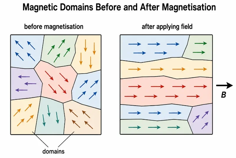
Ferromagnetic materials become magnetised when existing magnetic domains become more aligned with an applied magnetic field.
This diagram shows how magnetic domains in a ferromagnetic material change during magnetisation. Before magnetisation, the domains point in several different directions, so their magnetic effects partly cancel. After an external magnetic field B is applied, more domains align in the field direction, producing a stronger overall magnetisation. The illustration helps students understand that magnetisation occurs mainly through the alignment and growth of existing domains, not by creating magnetic behaviour from nothing.
Magnetic Susceptibility and Permeability Constants
Magnetic susceptibility describes the dimensionless scaling ratio that dictates how strongly a specific medium magnetises in response to an auxiliary field intensity driver:
$$\mathbf{M} = \chi_m \mathbf{H}$$
Where χm is the magnetic susceptibility parameter. A positive susceptibility value indicates that the material’s internal dipoles align constructively with the field, whereas a negative value defines a diamagnetic material that resists the flux lines.
Magnetic permeability measures the absolute capability of a substance to support and concentrate magnetic flux within its coordinates:
$$\mathbf{B} = \mu \mathbf{H}$$
Where μ is the absolute permeability of the medium (μ = μ0μr). Materials with exceptionally high relative permeability constants (μr >> 1) act as high-efficiency conduits that gather and direct magnetic flux lines along intended circuit pathways.
Industrial Applications: The Mechanics of Material Fields
Selecting specific magnetic responses is vital for engineering power conversion networks and quantum storage hardware:
High-Coercivity Permanent Magnets
Hard magnetic materials resist demagnetisation, providing steady fields inside electric vehicle motors, high-fidelity acoustic loudspeakers, and magnetic holding tools.
Low-Loss Transformer Cores
Soft magnetic materials switch their domain states with minimal hysteresis energy loss, guiding alternating magnetic flux efficiently through power transformer networks.
Super-Permeability Shielding
High-permeability materials (like Mu-Metal) act as path alternatives that redirect ambient magnetic interference completely around sensitive instrumentation cavities.
Non-Volatile Spintronic Storage
Nanoscale magnetic domain layers encode bit orientations via spin polarized currents, supporting advanced non-volatile computing architectures and dense memory arrays.
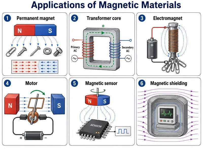
Magnetic materials are chosen for different devices according to how they retain, guide, strengthen, detect, or shield magnetic fields.
This infographic shows several important applications of magnetic materials. Permanent magnets retain magnetisation and attract magnetic objects. Transformer cores guide changing magnetic flux between primary and secondary coils. Electromagnets use current-carrying coils and magnetic cores to produce controllable magnetic fields. Motors use magnetic fields and current-carrying conductors to produce rotation. Magnetic sensors detect field changes and convert them into electrical signals. Magnetic shielding uses suitable materials to redirect magnetic field lines and protect sensitive equipment. The picture helps students connect magnetic dipoles, domains, magnetisation, and material response with real engineering devices.
Worked Examples with Step-by-Step Solutions
Worked Example 1: Magnetic Moment of a Single Loop Problem: A circular planar current loop encloses an area of 0.020 m² and carries a steady current of 3.0 A. Find the magnitude of its magnetic dipole moment. Solution: Apply the scalar dipole moment formula:
Answer: The magnetic dipole moment magnitude equals exactly 0.060 A·m², projecting perpendicular to the loop plane via right-hand parameters.
Worked Example 2: Magnetic Moment of a Multi-Turn Coil Problem: A compact inductor coil is wound with 50 turns over a cross-sectional area of 0.015 m². If it carries a direct current of 2.0 A, calculate its net dipole moment magnitude. Solution: Scale the baseline loop area equation by the turn count factor N:
Answer: The net magnetic dipole moment of the coil equals exactly 1.5 A·m².
Worked Example 3: Torque on an Oblique Dipole Problem: A magnetic dipole possessing a moment magnitude of 0.20 A·m² is placed inside a uniform 0.50 T magnetic field at an oblique angle of 30°. Calculate the mechanical torque acting on the dipole loop. Solution: Apply the scalar cross-product expansion equation:
Answer: The mechanical turning torque acting on the loop axis measures exactly 0.050 N·m.
Worked Example 4: Energy Configuration states Problem: A magnetic dipole loop holding a moment magnitude of 0.10 A·m² is placed in perfect parallel alignment with a uniform 0.40 T magnetic field. Calculate its potential energy. Solution: Apply the scalar dot product potential energy formulation:
$$U = -\boldsymbol{\mu}\cdot\mathbf{B} = -\mu B \cos\theta$$
Because the vectors are perfectly aligned parallel (θ = 0°), the cosine value equals 1:
Answer: The potential energy of the aligned dipole state equals exactly -0.040 J. The negative value indicates an energetically stable, favorable configuration.
Common Conceptual Misconceptions
The Monopole Cutting Myth
Misconception: If you slice a high-coercivity bar magnet directly across its center line, you can successfully isolate the North and South magnetic poles. Reality: Magnetic monopoles do not exist in classical electromagnetism (∇ · B = 0). Cutting a magnet simply cleaves the domain structure, resulting in two smaller complete dipoles, each with its own North and South poles.
The Universal Ferromagnetic Assumption
Misconception: Every single material object placed inside a strong external magnetic field is automatically attracted to the field lines. Reality: Diamagnetic substances (like copper and water) actively oppose incoming flux lines and experience a weak repulsive force, running completely counter to ferromagnetic attraction behaviors.
Quick Check: Magnetic Dipoles
Quick Check: Magnetic Dipoles
1. What is a magnetic dipole?
A magnetic dipole is a small magnetic system with a magnetic moment, such as a tiny current loop or an atomic magnetic moment.
2. What is the magnetic dipole moment of a single current loop?
For a single loop, the magnetic dipole moment has magnitude μ = IA, where I is current and A is loop area.
3. How is the direction of μ found for a current loop?
Use the right-hand rule. Curl your fingers in the direction of conventional current; your thumb points in the direction of the magnetic moment.
4. What happens to a magnetic dipole in an external magnetic field?
It experiences a torque that tends to rotate the dipole so that its magnetic moment aligns with the magnetic field.
Quick Check: Magnetic Materials
Quick Check: Magnetic Materials
1. What is magnetisation?
Magnetisation is the net magnetic dipole moment per unit volume inside a material.
2. What is the main difference between paramagnetic and ferromagnetic materials?
Paramagnetic materials align weakly with an applied field and usually lose the alignment when the field is removed. Ferromagnetic materials can align strongly and may retain magnetisation due to domain structures.
3. What are magnetic domains?
Magnetic domains are regions in a ferromagnetic material where many microscopic magnetic moments are aligned in roughly the same direction.
4. Why are soft magnetic materials useful in transformer cores?
They magnetise and demagnetise easily, which helps guide changing magnetic flux while reducing hysteresis energy loss.
Numerical Practice
Numerical Practice: Magnetic Dipoles
1. A single loop has area 0.030 m² and carries current 2.0 A. Find its magnetic dipole moment.
3. A dipole with μ = 0.30 A·m² is placed in a 0.40 T field at 90°. Find the torque magnitude.
Use τ = μB sin θ. Since sin(90°) = 1, τ = (0.30)(0.40) = 0.12 N·m.
4. A dipole with μ = 0.25 A·m² is aligned with a magnetic field of 0.80 T. Find its potential energy.
For alignment, U = –μB. Thus U = -(0.25)(0.80) = -0.20 J.
Review Questions and Answers
Review Questions: Magnetic Dipoles and Materials
1. Why can a current loop be treated as a magnetic dipole?
A current loop produces an external magnetic field configuration identical to that of a small bar magnet. It possesses a well-defined magnetic dipole moment vector μ = IAn̂.
2. What does the vector torque statement τ = μ × B physically demonstrate?
It states that a magnetic dipole resting inside an external field experiences a mechanical turning force that continuously rotates its dipole moment axis until it aligns parallel with the field lines.
3. Why are domain boundaries crucial in the study of ferromagnetic media?
Domains explain how vast populations of individual atomic moments align inside local zones. When an external field forces these separate zones to grow and merge along a single vector heading, the material develops intense macro-scale magnetisation.
4. What is magnetic hysteresis?
Hysteresis is the non-linear dependence of a material’s current magnetisation state on its prior magnetic field history, mapping out energy losses and retained field levels during cyclic magnetisation.
Thought-Provoking Questions
Thought-Provoking Questions
1. Why is a permanent bar magnet fundamentally mischaracterized when modeled as possessing distinct, isolated North and South magnetic charges?
Because magnetic fields are solenoidal (∇ · B = 0), meaning magnetic monopoles do not exist. Slicing a bar magnet simply cleaves the domain network, instantly producing two smaller, complete dipoles each containing their own North and South parameters.
2. Why do soft magnetic core alloys perform exceptionally well inside alternating-current machinery, whereas hard magnetic alloys are reserved for permanent magnets?
Soft magnetic alloys possess low coercivity values, meaning their domain walls shift with minimal resistance and heat loss during cyclic field reversals. Hard magnetic alloys feature extremely high coercivity, pinning domain walls securely in place to resist demagnetisation and maintain a persistent external field.
Glossary
Magnetic dipole: A basic closed magnetic infrastructure containing closely spaced, opposing virtual pole attributes, modeled mathematically as a current loop.
Magnetic dipole moment (μ): The operational vector quantity that measures the directional alignment heading and absolute mechanical torque capacity of a dipole system.
Magnetisation (M): A macroscopic vector field mapping the total net density of atomic magnetic dipole moments per unit volume inside a material continuum.
Diamagnetism: A weak, universal magnetic field response where electron orbital alterations construct tiny induced dipoles that directly oppose incoming external flux paths.
Paramagnetism: A weak magnetic attraction driven by the partial alignment of permanent atomic electron spins along external field vectors, rapidly neutralized by thermal agitation.
Ferromagnetism: An intense magnetic material state where quantum exchange interactions lock adjacent atomic spins into parallel alignment within macroscopic domain boundaries.
Magnetic domain: A microscopic localized pocket inside a ferromagnetic substance where all constituent atomic moments are aligned along a uniform direction.
Hysteresis: The non-linear lagging behavior of a material’s magnetization curve relative to an oscillating external magnetic intensity drive.
Coercivity: The measurement threshold tracking the intensity of a reverse external magnetic field required to reduce a magnetized material’s residual flux density back to zero.
Permeability (μ): The scalar media constant tracking how easily a material continuum concentrates and supports incoming lines of magnetic flux density.
Magnetic dipoles and materials map out the physical parameters dictating how condensed matter responds to external magnetic field paths. A singular current-carrying circuit loop mimics a magnetic dipole, establishing a vector dipole moment defined by μ = IAn̂. When immersed in an external magnetic flux landscape, the dipole experiences an orthogonal mechanical torque (τ = μ × B), turning until its potential energy configuration states are minimized. Within bulk matter, millions of these fractional atomic spins combine to project a macroscopic magnetisation vector field M.
Depending on internal electron sub-shell layouts and exchange interactions, material families separate into diamagnetic, paramagnetic, ferromagnetic, ferrimagnetic, and antiferromagnetic categories. Ferromagnetic media stands out as critically important due to the presence of internal magnetic domains and multi-valued hysteresis profiles, which allow engineers to explicitly designate hard or soft magnetic core behaviors for distinct technology fields.
For university engineering preparation, the essential lesson is that materials cannot be simply lumped into binary “magnetic” or “non-magnetic” descriptions. Their real-world utility depends on analyzing underlying atomic dipole states, tracking domain wall movements under stress, and exploiting susceptibility changes to guide, strengthen, modulate, or block magnetic fields systematically.
Reflection Question
If the macro-scale magnetism of a permanent magnet or transformer core originates from the collective alignment and movement of millions of microscopic magnetic domains and quantum electronic spins, how does this fluid, domain-based reality reframe your mechanical perception of solid, static iron machinery?