Prepare for University Studies & Career Advancement
Biot–Savart Law: Magnetic Fields from Currents
The Biot–Savart law represents the fundamental, element-based mathematical framework governing how moving electrical charges generate magnetic fields. It stands as the direct magnetic analog to Coulomb’s law in electrostatics, serving as the primary diagnostic tool in classical magnetostatics—the study of time-independent magnetic environments driven by steady currents. Instead of attempting to parse an entire arbitrary conductor layout at once, the Biot–Savart formulation abstracts the system down to an infinitesimal current element, computing its differential magnetic flux density contribution at any given point in coordinate space.
This differential resolution provides the law with its immense analytical power. Any geometric layout—whether it is a simple straight conductor segment, a circular loop, a multi-turn induction coil, or an asymmetric industrial wire matrix—can be mathematically modeled as a continuous line continuum of individual current elements acting together. Each element contributes a fractional magnetic vector to the local environment, and the true total magnetic field is extracted by executing a vector summation over the entire conductor contour.
For undergraduate physics students and electrical engineers transitioning to advanced electromagnetic field theory, mastering the Biot–Savart law represents a major conceptual leap. It replaces vague notions of fields being vaguely “around wires” with a rigid, vector-based framework. It demonstrates that steady magnetic fields are precise geometric products of moving charge magnitudes, shaped continuously by spatial orientation angles, and mapped strictly through cross-product directional matrices.
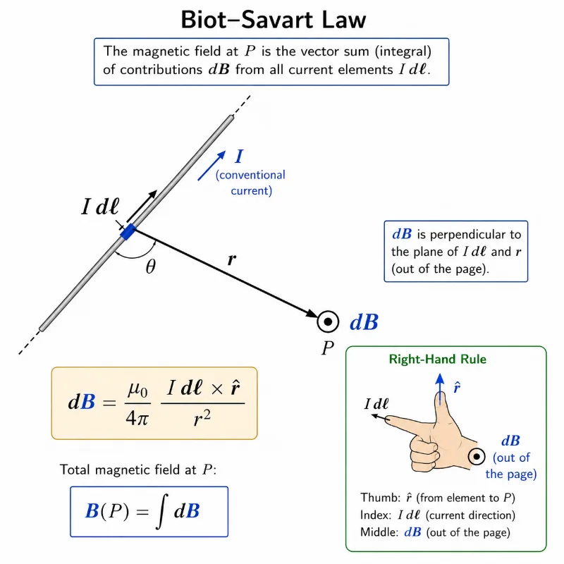
A small current element contributes a small magnetic field dB at point P, with the direction determined by the right-hand rule.
This illustration introduces the Biot–Savart law by showing how a tiny current element I dℓ on a wire contributes to the magnetic field at a nearby point P. The displacement vector r points from the current element to the observation point, while the angle θ shows the geometry between the current direction and the line to P. The magnetic field contribution dB is shown perpendicular to the plane formed by I dℓ and r, represented as coming out of the page. The right-hand-rule inset helps students connect the vector cross product with the physical direction of the magnetic field contribution.
Learning Pathway
This module serves as the primary element-based entry point for the Magnetostatics cluster under the global Electricity and Magnetism curriculum. It establishes the foundational superposition principles required before students advance to symmetry-based line integrals (Ampère’s Law) and the macroscopic magnetic boundary behaviors of real materials.
Provides the global parent context for understanding charge distributions, vector field equations, electric circuits, induction, and Maxwellian wave mechanics.
Introduces how steady, time-independent currents configure local space to generate constant magnetic fields and establish forces across material systems.
The Biot–Savart Law
Evaluates magnetic fields by executing brute-force differential integrations along arbitrary, non-symmetrical current-carrying line contours.
Deploys closed line integrals and spatial symmetry profiles to extract exact magnetic field values for regular, uniform current distributions without direct integration.
Analyzes atomic magnetic moments, domain boundaries, magnetization vectors, and how materials alter ambient flux paths.
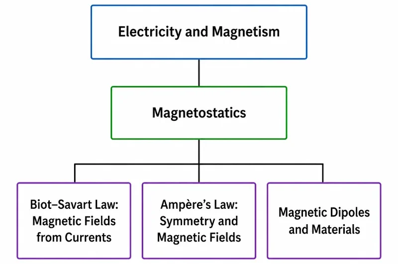
This hierarchy chart shows Magnetostatics within Electricity and Magnetism, with three focused pages on magnetic fields from currents, symmetry-based magnetic field calculation, and magnetic dipoles in materials.
This simple tree chart presents the Magnetostatics cluster within the wider Electricity and Magnetism section of Prep4Uni.online. Electricity and Magnetism appears as the parent area, followed by Magnetostatics as the hub page. The three child pages are Biot–Savart Law: Magnetic Fields from Currents, Ampère’s Law: Symmetry and Magnetic Fields, and Magnetic Dipoles and Materials. The chart helps students see how the Magnetostatics pathway moves from current elements and magnetic field calculation to symmetry methods and the magnetic behaviour of matter.
What the Biot–Savart Law Really Means
The Biot–Savart law functions as the exact magnetostatic counterpart to the field-building concepts utilized in electrostatics. When computing electric fields, a complex charge distribution is broken into infinitesimal point charges, and their individual electric field vectors are summed up. In magnetostatics, a complex current network is similarly broken down into localized current element paths, and their individual magnetic field contributions are calculated.
However, a critical difference emerges in the vector geometry. While electrostatic fields point radially along the line of sight connecting the source charge to the observation point, magnetostatic fields act purely sideways. Their direction is governed by a vector cross product, which forces the field lines to project perpendicularly to both the direction of the moving charges and the line of sight vector. This orthogonal relationship makes magnetic fields less intuitive initially, but exceptionally interesting from a geometric modeling perspective.
Mastering the Biot–Savart framework relies on two rigid analytical habits: first, splitting a continuous current system into discrete, directed elements; and second, treating each fractional contribution as a true vector quantity possessing an explicit magnitude and orientation. The absolute field value at the target coordinate is the definitive vector sum of every single piece along the path.
The Vector and Scalar Formulations
Mathematically, the differential magnetic flux density contribution generated by an infinitesimal current element is defined by the vector cross-product equation:
Where dB is the fractional magnetic field vector, I matches the steady current magnitude, dℓ represents the infinitesimal length vector tangent to the conventional current path, r̂ is the unit vector pointing from the source element coordinates directly toward the observation target, and r is the scalar distance separating those two spatial positions. To extract the pure scalar magnitude of this contribution, the cross product is expanded into its angular form:
Where θ tracks the exact geometric angle evaluated between the current direction vector dℓ and the line of sight displacement vector.
Deconstructing the Equation Blocks
To successfully deploy the Biot–Savart equation across varying coordinate systems, each standalone term must be rigorously analyzed:
Steady Current (I)
Measures the quantity of electric charge passing through a cross-section of the conductor per second. The resulting magnetic field strength scales in direct linear proportion to this current flux.
Length Vector (dℓ)
Represents the infinitesimal directed segment of the wire path. Its orientation points along the direction of conventional current, rather than electron drift velocity.
Line of Sight Unit Vector (r̂)
A dimensionless directional pointer originating at the specific current element coordinates and pointing directly at the observation point where the field is being calculated.
Inverse Square Term (r²)
Dictates the spatial decay of the magnetic interaction. As the distance from a current element increases, its field contribution weakens exponentially, following an inverse-square law.
Angular Modifier (sin θ)
Tracks the directional orientation of the current element. Only the component of the moving charge vector running perpendicular to the line of sight generates a magnetic field at that point.
Vacuum Permeability constant (μ0)
Establishes the fundamental magnetic scaling constant in a vacuum, holding an exact value of 4π × 10-7 T·m/A.
The Geometric Consequence of Cross Products
The vector cross product dℓ × r̂ completely controls the directional profile of the magnetic field. By vector rules, the resulting dB vector must project at a strict right angle to the plane formed by the current element and the line of sight vector. This explains why the magnetic field lines around a long straight wire form concentric, closed circular loops instead of radiating straight outward. The field never points away from the wire, and it never points along the wire axis; it encircles the conductor continuously.
To quickly find this direction in practice, use the **Right-Hand Rule for Current Elements**: point your right thumb straight along the direction of conventional current flow. Your curled fingers then indicate the circular direction of the magnetic field lines encircling the conductor path.
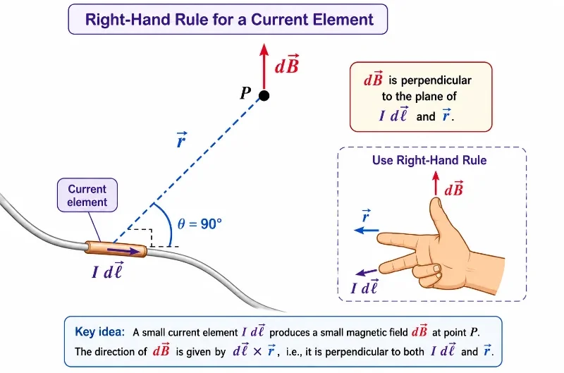
The right-hand rule shows that the magnetic field contribution dB from a current element is perpendicular to both the current element I dℓ and the position vector r.
This illustration explains the right-hand-rule direction used in the Biot–Savart law. A small current element I dℓ is shown on a wire, with a position vector r pointing from the current element to point P, where the magnetic field is being considered. The magnetic field contribution dB is drawn perpendicular to both I dℓ and r, highlighting the orthogonal relationship expressed by the cross product. The hand diagram reinforces the idea that the direction of dB is not along the wire and not along r, but perpendicular to the plane formed by them.
Evolution of Current Trajectory Physics: History, Challenges, and Frontiers
To establish a comprehensive understanding of magnetostatic field theory, it is essential to trace how the Biot–Savart law evolved, its contemporary engineering challenges, and its future application boundaries.
Historical Epochs: From Oersted’s Compass to the Formalization of Field Integration
The quantitative era of magnetic field physics was ignited in the spring of 1820, when Danish natural philosopher Hans Christian Ørsted observed that an active electrical current deflected a nearby compass needle, providing the first concrete proof linking electricity and magnetism. Within months of learning about Ørsted’s discovery, French physicists Jean-Baptiste Biot and Félix Savart conducted meticulous experiments with thin wires to measure how forces varied with distance. By late 1820, they formulated the exact differential expression detailing how a fractional current element projects a magnetic field vector into space. Pierre-Simon Laplace later generalized this relation into its complete integral calculus form, allowing scientists to transition from simple experimental measurements to a mathematically rigorous theory of vector fields.
Contemporary Engineering Challenges: Managing Non-Symmetrical Fields in Complex Infrastructure
While applying the Biot–Savart equation to ideal straight lines or circular loops is algebraically elegant, real-world electrical infrastructure rarely possesses perfect coordinate symmetry. In high-power distribution grids, electronic circuit boards, and industrial transformers, current paths are twisted, finite, and non-uniform. Because simple loop approximations break down in these systems, engineers face **flux leakage** and localized electromagnetic interference (EMI). Predicting these stray fields requires solving the Biot–Savart integral through brute-force numerical integration and high-fidelity finite element analysis (FEA). These computational methods are vital for optimizing magnetic shielding and ensuring electromagnetic compatibility across sensitive communication equipment.
Future Technological Horizons: Micro-Coil Magnetic Traps and Quantum Spintronics
Today, the foundational vector mechanics of the Biot–Savart law are driving innovations at the cutting edge of quantum computing and nanotechnology. In atomic physics research, engineers design micro-fabricated wire arrays on chips to create precise **Magnetic Traps**. By running controlled direct currents through custom geometric paths, they create highly localized magnetic fields that can trap and cool individual neutral atoms or ions without physical contact, providing a stable platform for quantum bits (qubits). Simultaneously, the field of **spintronics** is moving beyond standard bulk current paths to utilize localized, spin-polarized current streams at the nanoscale. Modeling the incredibly tight, highly non-uniform magnetic signatures generated by these sub-micron spin flows relies on advanced applications of the Biot–Savart law, enabling next-generation non-volatile memory chips with near-zero energy loss.
Integrating Along a Continuous Conductor
Because a physical conductor is composed of an infinite continuum of individual current elements, finding the absolute net magnetic field at any point in space requires executing a line integral over the entire active current contour C:
This vector integration is the mathematical equivalent of summing an infinite number of tiny fractional arrows. In highly symmetrical configurations, spatial coordinate symmetries allow the vector components to be simplified, making the integration straightforward. In complex, asymmetric arrangements, the equation must be solved piece-by-piece using numerical algorithms on a computer.
Advanced Derivation Case Study: The Axial Loop Configuration
To understand how the Biot–Savart law handles vector components during integration, consider a single circular wire loop of radius R carrying a steady current I, placed symmetrically in the xy-plane. We want to find the exact magnetic field vector at an observation point P located a distance z along the central perpendicular axis of the loop.
Let dℓ be an infinitesimal current element on the loop circumference. The line of sight vector pointing from this element to point P forms a right-angled triangle with the radius R and the axial distance z, establishing the distance relationship:
$$r = \sqrt{R^2 + z^2}$$
Crucially, because the circular path curls perfectly around the central axis, every current element dℓ is exactly perpendicular to its respective line of sight unit vector r̂ (θ = 90°), which simplifies the scalar cross-product magnitude because sin(90°) = 1:
Now, analyze the vector orientation of this differential field contribution dB. By the right-hand rule, dB projects at a right angle to the line of sight vector, meaning it tilts away from the central axis by an angle φ. When integrating around the complete circular loop, the perpendicular components of the field rotate around the axis and cancel out completely due to symmetry. Only the parallel axial components survive the loop integration:
$$dB_z = dB \cos\phi$$
From the geometry of the right-angled triangle, the cosine of the tilt angle is defined as $ \cos\phi = R / r = R / \sqrt{R^2 + z^2} $. Substituting this geometric relation into the axial force component equation yields:
Because every parameter except the differential length element dℓ is constant at a fixed distance along the axis, they can be pulled entirely outside the integral. Integrating dℓ around the loop circumference yields the circle’s total perimeter ($ 2\pi R $):
$$B_z = \frac{\mu_0 I R}{4\pi (R^2 + z^2)^{3/2}} \oint d\ell = \frac{\mu_0 I R}{4\pi (R^2 + z^2)^{3/2}} \cdot (2\pi R)$$
Simplifying the scalar fractions results in the definitive axial loop field equation:
$$B_z = \frac{\mu_0 I R^2}{2(R^2 + z^2)^{3/2}}$$
To find the field strength at the exact center of the loop, set the axial distance to zero (z = 0). The equation simplifies directly to the classical circular loop formula:
$$B = \frac{\mu_0 I R^2}{2(R^2)^{3/2}} = \frac{\mu_0 I}{2R}$$
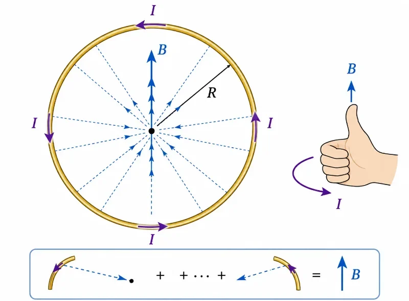
A circular current loop produces a magnetic field through its centre, with the direction determined by the right-hand rule.
This illustration shows how a circular wire loop carrying current produces a magnetic field at its centre. The current I flows around the loop, while the radius R marks the distance from the centre to the wire. The magnetic field B through the centre results from the combined contributions of all small current elements around the loop. The right-hand-rule cue helps students see how the direction of current around the loop determines the direction of the magnetic field through the centre.
Field Profile of a Semicircular Conductor Arc
For a fractional circular arc subtending an arbitrary angle φ (measured in radians) with a radius R, integrating the scalar Biot–Savart equation yields:
$$B = \frac{\mu_0 I \phi}{4\pi R}$$
This result demonstrates how full geometric orbits are constructed from fractional elements. For example, a complete circular loop subtends a full angle of 2π radians; substituting $ \phi = 2\pi $ into the arc equation simplifies directly to the standard circular loop formula ($ B = \mu_0 I / 2R $), proving the mathematical consistency of the field-building method.
Field Profile Outside an Infinite Straight Wire
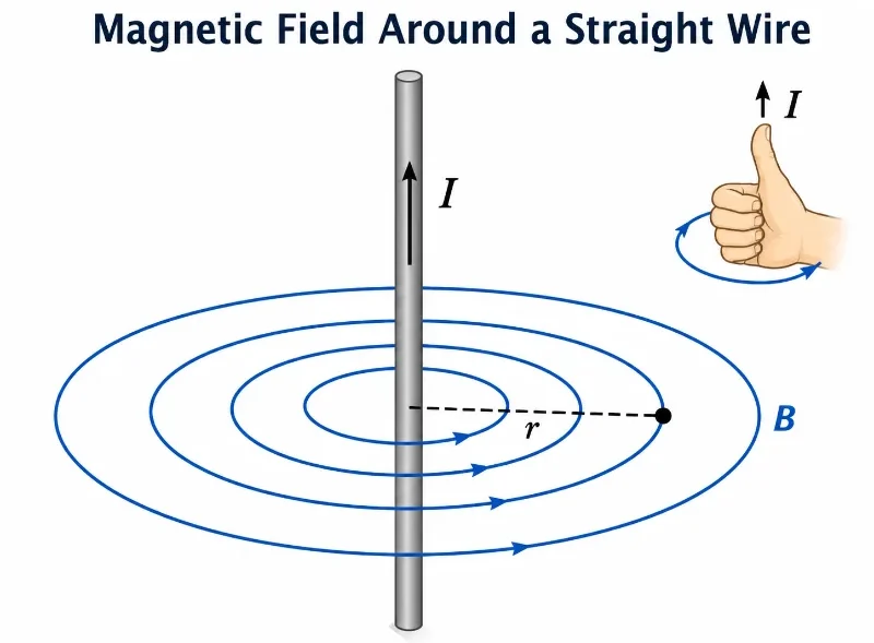
Integrating the differential element equations along an infinitely long straight wire shows that the magnetic field strength at a perpendicular distance r from the wire axis is described by:
$$B = \frac{\mu_0 I}{2\pi r}$$
The field strength scales in direct proportion to the current and decays inversely with distance from the wire, mapping out as closed circular loops encircling the conductor path.
A straight wire carrying current produces circular magnetic field lines around the wire, with the direction given by the right-hand rule.
This illustration shows the magnetic field produced by a straight current-carrying wire. The current I flows upward through the vertical wire, while the blue circular field lines show the magnetic field B surrounding the wire. The distance r marks how far the observation point is from the wire. The right-hand-rule cue reminds students that when the right thumb points in the direction of conventional current, the curled fingers show the circular direction of the magnetic field. The diagram helps students understand why the magnetic field does not point straight outward from the wire, but forms closed loops around it.
Biot–Savart Law versus Ampère’s Circuital Law
While the Biot–Savart law and Ampère’s law both calculate magnetic fields generated by steady electrical currents, their analytical application strategies differ completely:
The Biot–Savart Integral Law
Builds up fields by summing individual differential contributions from current line elements. It serves as the primary tool for computing fields around finite wires, broken loops, arcs, and arbitrary, non-symmetrical current paths.
Ampère’s Circuital Law
Binds the field circulation along a path directly to the total enclosed free current. It is incredibly efficient for solving highly symmetric current layouts, bypassing difficult multi-dimensional vector integration completely.
The Optimal Design Choice
Implement Ampère’s circuital integrals when high spatial symmetry allows the field parameter to be factored out cleanly. Use the Biot–Savart differential law when the system’s geometric profile breaks coordinate uniformity.
Industrial Applications: The Mechanics of Geometric Fields
Connecting current geometries to exact magnetic field maps is the operational foundation of advanced electrical engineering and scientific instrument design:
Power Transmission Lines
The law models and maps electromagnetic fields around industrial distribution cables, helping engineers minimize cross-talk and optimize electromagnetic compatibility.
Precision Inductive Coils
Multi-layer inductive loops and electromagnetic chokes are engineered by calculating how many winding turns are needed to generate specific magnetic field intensities.
Solid-State Magnetic Sensors
High-sensitivity Hall-effect and magnetoresistive sensors rely on exact field calculations to detect positions, track mechanical motion, and measure current signatures safely.
Scientific Particle Guidance Instruments
Mass spectrometers, electron microscopes, and particle accelerators use precisely wound wire paths to create custom fields that steer or trap charged particle beams without physical contact.
The Biot–Savart law helps connect current geometry with magnetic field patterns in wires, coils, sensors, electromagnets, laboratory experiments, and scientific instruments.
This infographic shows several practical applications of the Biot–Savart law. It illustrates magnetic field lines around current-carrying wires, stronger fields produced by coils and solenoids, magnetic sensors detecting field changes, laboratory experiments comparing measured and predicted magnetic fields, electromagnets producing useful attraction, and scientific instruments using magnetic fields to guide or bend charged particles. The picture helps students see that the Biot–Savart law is not only a mathematical rule, but a way to understand how current geometry shapes magnetic fields in technology, experiments, and engineering design.
Worked Examples with Step-by-Step Solutions
Worked Example 1: Field Outside a Long Straight Wire Problem: A long straight wire carries a steady current of 5.0 A. Calculate the magnetic flux density at an observation point located a perpendicular distance of 0.10 m from the wire center. Solution: Apply the infinite straight line conductor equation:
Answer: The magnetic field strength equals exactly 1.0 × 10⁻⁵ T, mapping circularly around the wire via the right-hand rule.
Worked Example 2: Field at the Center of a Circular Loop Problem: A single circular wire loop of radius 0.050 m carries a steady current of 3.0 A. Find the magnetic field strength at the exact center of the loop. Solution: Apply the circular loop center equation (derived by setting z = 0 in the axial formula):
Answer: The magnetic field at the center of the loop measures approximately 3.77 × 10⁻⁵ T.
Worked Example 3: Field at the Center of a Multi-Turn Coil Problem: A compact multi-turn coil contains 20 identical turns of wire wound with a mean radius of 0.080 m. If it carries a current of 2.5 A, estimate the magnetic field strength at its center. Solution: Scale the loop center equation by the total number of turns N:
Answer: The magnetic field at the center of the coil measures approximately 3.93 × 10⁻⁴ T.
Worked Example 4: Field from a Semicircular Arc Problem: A wire is bent into a semicircular arc of radius 0.080 m and carries a current of 2.0 A. Calculate the magnetic field contribution at the center of curvature originating solely from this arc. Solution: Apply the circular arc equation using a semicircular angle of exactly π radians:
$$B = \frac{\mu_0 I \phi}{4\pi R} \Rightarrow B = \frac{\mu_0 I \pi}{4\pi R} = \frac{\mu_0 I}{4R}$$
Answer: The magnetic field contribution from the semicircular arc measures approximately 7.85 × 10⁻⁶ T.
Common Conceptual Misconceptions
The Radial Force Fallacy
Misconception: The magnetic field vectors point straight out radially away from the current element, similar to electrostatic field lines. Reality: The direction is governed by a vector cross product, forcing the field lines to project strictly perpendicular to the line of sight and forming closed circular loops encircling the wire path.
The Scalar Summation Trap
Misconception: You can find the total magnetic field of a wire by simply integrating the scalar magnitudes of each element’s field contribution. Reality: The Biot–Savart law is fundamentally a vector relationship. Field contributions must be added as vectors; components that point in opposite directions can cancel out completely due to symmetry, altering the final field strength.
Quick Check: Meaning of the Biot–Savart Law
Quick Check: Meaning of the Biot–Savart Law
1. What does the Biot–Savart law calculate?
It calculates the magnetic field produced by electric current. More precisely, it gives the small magnetic field contribution from a small current element, and the total field is found by adding all contributions.
2. Why is the Biot–Savart law a vector law?
Because each magnetic field contribution has both magnitude and direction. The direction is determined by the cross product dℓ × r̂.
3. What happens to the magnetic field contribution when the observation point is farther away?
The contribution becomes smaller because the Biot–Savart law contains the inverse-square factor 1 / r².
4. Why does sin θ appear in the magnitude form?
It appears because only the part of the current element perpendicular to the direction toward the observation point contributes to the magnetic field magnitude.
Quick Check: Direction and Right-Hand Rule
Quick Check: Direction and Right-Hand Rule
1. Around a straight wire carrying current upward, what shape are the magnetic field lines?
The magnetic field lines form circles around the wire.
2. Which direction should your right thumb point when using the right-hand rule for a straight wire?
Your right thumb should point in the direction of conventional current. Your curled fingers then show the direction of the magnetic field around the wire.
3. If the current in a wire is reversed, what happens to the magnetic field direction?
The magnetic field direction reverses. The circular field lines still surround the wire, but their circulation direction changes.
Glossary
Biot–Savart law: A fundamental magnetostatic law that defines the differential magnetic flux density contribution generated by an infinitesimal current element.
Current element: An infinitesimal vector segment of a current path, mathematically expressed as I dℓ.
Observation point: The specific coordinate location in space where the net magnetic field vector is being evaluated.
Right-hand rule: A geometric visualization rule used to find cross-product vector directions based on the orientation of the right hand.
Magnetic field (B): A solenoidal vector field generated by moving electrical charges, steady currents, or intrinsic atomic magnetic moments.
Vacuum permeability (μ0): The fundamental scalar scaling constant anchoring magnetic field metrics within free space environments.
Superposition: The physical principle stating that the net field at any point equals the vector sum of all individual field contributions.
Magnetostatics: The branch of electromagnetic theory that analyzes time-independent magnetic fields driven by steady currents.
Magnetic field line: A visual vector map line whose tangent at any point indicates the exact direction of the local magnetic field.
Current loop: A closed conducting loop path carrying current, widely engineered to project a uniform magnetic field through its center.
The Biot–Savart law describes how steady electrical currents generate time-independent magnetic fields. It breaks down a conducting circuit into infinitesimal current elements, calculating the fractional magnetic flux density vector contributed by each element. Mathematically, this relation is governed by the vector cross-product equation dB = (μ0 / 4π) · (I dℓ × r̂ / r²).
The law is exceptionally powerful because it builds complex magnetic field maps through the principle of vector superposition. Any wire contour, circular loop, fractional arc, or winding coil can be modeled as a continuous line continuum of individual elements whose field vectors are integrated over the entire path length.
The most critical diagnostic lesson is that magnetic field distributions depend heavily on current magnitudes, inverse-square distances, and the orientation angle between the current path and the line of sight. Utilizing the right-hand rule is essential because the spatial direction of the field vector is derived entirely from a vector cross product.
For university preparation, mastering the element-based Biot–Savart law establishes the essential mathematical foundation needed before students transition to symmetry-based line integrals (Ampère’s Law) and advance to modeling macroscopic field lines inside magnetic materials.
Reflection Question
If the total magnetic field at an observation point can be built up by summing the independent vector contributions from an infinite number of tiny current elements along a wire, how does this atomic, field-building perspective change the way you physically visualize the space surrounding active electrical machinery?