
Electric potential and voltage enable university-level students to transition from simple Newtonian mechanics to sophisticated energy conservation paradigms. While an electric field quantifies the localized vector force exerted per unit charge, electric potential abstracts the electrostatic environment into a continuous scalar field that defines the exact amount of electrostatic potential energy available per unit charge at any given coordinate point.
This represents a powerful paradigm shift in physical reasoning. Instead of calculating vector components to ask, “Which direction is a particle pushed?”, we analyze scalar distributions to determine the net energy state an object possesses purely due to its geometric location. Voltage, or electric potential difference, defines the path-independent energy change per unit charge between two distinct coordinates, directly linking microscopic electrostatics to practical circuit components, macro-scale batteries, and high-energy particle accelerators.
Main Picture
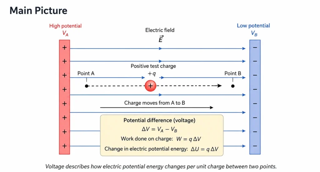
This illustration shows a positive test charge moving between two points in a uniform electric field. Point A is at higher electric potential, while point B is at lower electric potential. As the charge moves through the potential difference, its electric potential energy changes according to the voltage between the two points. The diagram helps students understand that voltage is not simply a number printed on a battery; it is a measure of energy change per unit charge.
Learning Pathway in Electricity and Magnetism
Electricity and Magnetism
Introduces the overarching academic domain governing electric and magnetic phenomena, spanning static charges, dynamic currents, magnetic induction, and Maxwellian systems.
Electrostatics Parent Hub
Provides the primary conceptual umbrella, focusing on static charge systems in structural equilibrium and their associated field and potential distributions.
Electric Charge and Coulomb’s Law
Establishes the initial quantitative entry point, defining charge quantization, tribal interactions, and the primary inverse-square force equations.
Electric Fields and Field Lines
Advances past dual-source force tracking to map space as a continuous vector field modified by isolated source charges.
Electric Potential and Voltage
Moves from electric field strength to energy per unit charge, helping students understand voltage as a physical energy idea.
Capacitance and Dielectrics
Applies field mappings and potential integrations to material polarization boundaries, physical hardware capacitors, and volumetric energy density metrics.
The Core Physical Idea
Electric Potential as Energy per Unit Charge
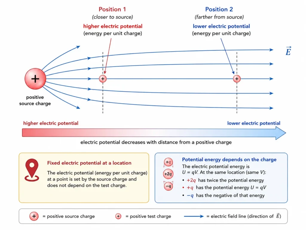
This illustration shows a positive source charge creating an electric field, with a positive test charge shown at two different positions. The position closer to the source charge has higher electric potential, while the position farther away has lower electric potential. The diagram helps students distinguish electric potential from electric potential energy: electric potential is the energy per unit charge at a location, while the actual potential energy depends on the particular charge placed there.
Voltage as a Difference Between Two Points
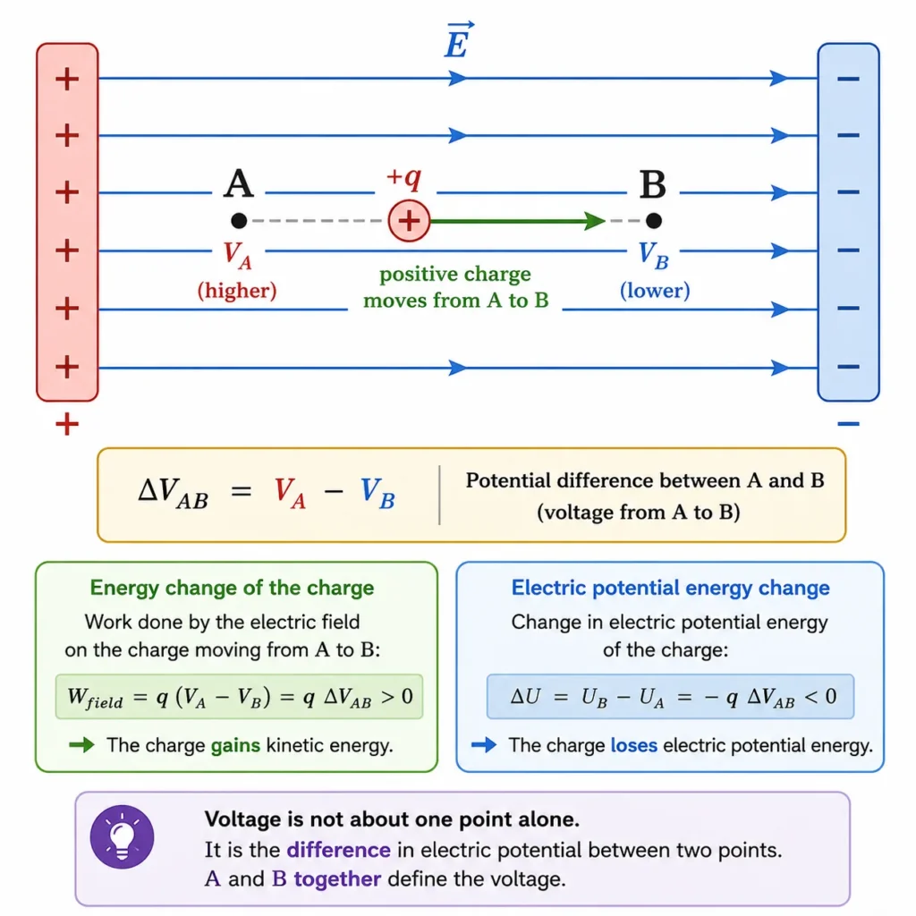
This illustration shows two points, A and B, in a uniform electric field between oppositely charged plates. Point A is at higher electric potential and point B is at lower electric potential. A positive charge moves from A to B, showing that voltage is not usually about one point alone but about the difference in electric potential between two locations. The image helps students see that when a charge moves through a potential difference, it may gain kinetic energy while its electric potential energy changes.
Equipotential Lines and Electric Field Direction
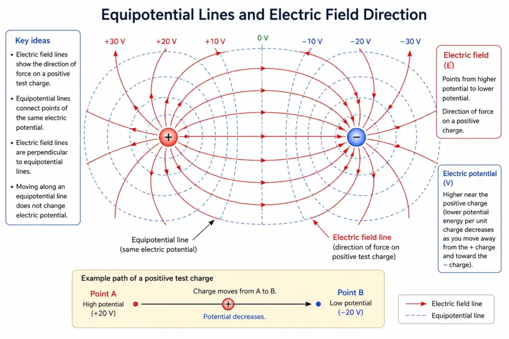
This illustration shows two connected visual ideas in electrostatics: electric field lines and equipotential lines. The electric field lines show the direction of force on a positive test charge and point from higher potential toward lower potential. The equipotential lines connect points with the same electric potential, so moving along one of these lines does not change electric potential. The diagram helps students see that, in a simple electrostatic case, electric field lines cross equipotential lines at right angles.
The Primary Pillar to Remember
Voltage is an absolute expression of electrical potential energy difference normalized per unit charge; it tracks the exact work potential across spatial coordinates.
Visualizing the Scalar Landscape
Map Normalized Potential Energy
Envision the electric potential as a standard structural blueprint map of the environment. It outlines exactly how much energetic pressure awaits any courier of charge entering that coordinate node.
Evaluate Path-Independent Differences
Voltage requires comparing two unique coordinates. It calculates the net work potential across a spatial gap, completely independent of the route or pathway chosen to travel between them.
Trace Gradient Vector Falls
Visualize vector electric field lines as paths running straight down potential hills. By rule, the field lines point directly along the direction of steepest potential decline.
Correlate Voltage Transmissions
Track the active energy transfer occurring across a potential drop. This conversion converts electrical potential energy into kinetic particle acceleration or circuit work.
Key Equations and Physical Interpretations
Physical Meaning of V = U / q
Electric potential isolates the base energetic capacity of a coordinate location. It removes the size parameter of the test charge to map systemic fields purely as energy topography.
The Operational Delta Rule
Voltage quantifies the work potential per unit charge across boundaries. It links electrical properties to classic thermodynamic work and energy transformations.
Linear Radial Decay Behavior
Unlike point-source vector fields which drop off quadratically (1/r²), scalar point potential fields drop off linearly (1/r). This difference impacts field integrations across spatial distributions.
From Formula to Meaning
Advanced Mathematical Rigor: Line Integrals of Conservative Vector Fields
Worked Analytical Example
- Net Charge magnitude (q) = 3.0 C
- Potential Energy gain (ΔU) = 18 J
Technical Case Studies: Potential Fields in Applied Technology
Macroscopic Energy Logistics: High-Voltage DC Transmission
Long-distance electrical grids use high-voltage DC (HVDC) transmission lines operating at potential differences exceeding 500,000 V to minimize power losses. Because power loss in a conductor depends on current squared ($I^2R$), grid engineers use extreme voltages to deliver massive energy quantities at very low current values. Elevating the potential energy per unit charge allows power companies to transmit megawatts of electrical energy across continents with minimal heat loss.
Micro-Particle Trajectory Symmetries: Cathode Ray Cathodes
Precision manufacturing instruments—such as scanning electron microscopes and legacy display tubes—rely on focused potential differences to accelerate subatomic particles. Electrons are released from a negative cathode assembly and pulled toward a positive anode block held at a high relative potential difference ($V = U/q$). As they cross this potential gradient, the electrons convert their potential energy near-instantaneously into directed kinetic energy, producing a highly focused electron beam.
Evolution of Potential Theory: History, Engineering Hurdles, and Future Frontiers
Historical Epochs: The Transition to Energy Field Paradigms
Contemporary Challenges: Managing Parasitic Gradients in Nanometer Semiconductors
Future Technological Horizons: Solid-State Electrochemical Potentials
Numerical Problems and Solutions
-
A charge of 4.0 C gains 20 J of electric potential energy when moved through an electric field. Find the potential difference.Solution: Apply the operational potential difference formula:$$\Delta V = \frac{\Delta U}{q} \Rightarrow \Delta V = \frac{20\text{ J}}{4.0\text{ C}} = 5.0\text{ V}$$Interpretation: The potential difference measures 5.0 V, meaning the moving charge scales its energy state by 5.0 Joules per individual coulomb.
-
A potential difference of 12 V is maintained across a circuit element. Calculate the total potential energy transferred when a net charge magnitude of 3.0 C passes through the component.Solution: Isolate the energy parameter from the voltage relationship:$$\Delta U = q\Delta V \Rightarrow \Delta U = (3.0\text{ C})(12\text{ V}) = 36\text{ J}$$Interpretation: The circuit element converts 36 Joules of electrical potential energy into heat or mechanical work as the charge carrier stream passes through.
-
An isolated point source charge carrying a value Q = +2.0 × 10⁻⁶ C establishes a scalar potential field in space. Compute the absolute potential at a radial coordinate distance r = 0.30 m from the source center.Solution: Deploy the inverse-distance scalar potential model:$$V = k_e \frac{Q}{r} \Rightarrow V = (8.99 \times 10^9) \frac{2.0 \times 10^{-6}\text{ C}}{0.30\text{ m}} \approx 6.0 \times 10^4\text{ V}$$Interpretation: The positive source creates a local potential capacity of 60,000 V at the 0.30 m boundary, using infinity as the absolute zero-potential reference point.
-
A uniform electric field maintains a steady field intensity of 500 N/C between two parallel plates. Determine the potential difference across a separation gap distance of 0.20 m along the field line vectors.Solution: Apply the linear field-to-potential mapping equation:$$|\Delta V| = Ed \Rightarrow |\Delta V| = (500\text{ N/C})(0.20\text{ m}) = 100\text{ V}$$Interpretation: The potential drop across the plates measures 100 V. By definition, the electric potential decreases directly along the pointing vectors of the field lines.
-
An electron carrying an elementary charge value e = 1.60 × 10⁻¹⁹ C accelerates through an electric potential drop of 50 V. Calculate the absolute energy change in Joules.Solution: Evaluate the transformation using particle charge metrics:$$|\Delta U| = q|\Delta V| \Rightarrow |\Delta U| = (1.60 \times 10^{-19}\text{ C})(50\text{ V}) = 8.0 \times 10^{-18}\text{ J}$$Interpretation: The single subatomic particle undergoes an energy conversion of 8.0 × 10⁻¹⁸ Joules, which scales it to an exact energy kinetic state of 50 electron-volts (eV).
Common Conceptual Misconceptions
The Fluid Volume Illusion
Misconception: High voltage profiles automatically prove that a system contains a massive quantity of electric charge.
Reality: Voltage tracks energy efficiency ratios (J/C), not charge volumes. A small static spark can carry thousands of volts of potential while moving only a few nanocoulombs of charge.
Potential vs. Potential Energy Confusion
Misconception: Electric potential is identical to electric potential energy.
Reality: Potential maps the background field location independently (V = U/q). The actual potential energy (U = qV) requires placing a specific charge value onto that coordinate map.
Applications of Electric Potential and Voltage
Chemical Battery Cells
Batteries maintain steady potential differences across their terminals, providing the continuous electrical pressure needed to drive current through circuit devices.
Hardware Capacitor Storage
Capacitors preserve potential energy by maintaining stable voltage drops across isolated conducting boundary layers.
Controlled Power Supplies
Electronic power supplies regulate potential drops, ensuring delicate microprocessors receive stable, fine-tuned voltages.
Lightning Strike Discharges
Massive potential differences between clouds and the ground build extreme field intensities that rip electrons from air molecules, causing a violent lightning discharge.
Real-World Engineering Integration
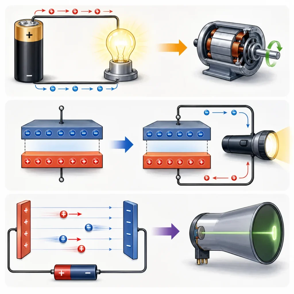
This illustration shows how voltage appears in real electrical systems. A battery can drive charge through a circuit to light a lamp or power a motor, a capacitor can store and release electrical energy, and charged particles can be accelerated through a potential difference. These examples help students understand that voltage is not only an abstract number; it describes how much energy is available per unit charge as electrical systems store, release, or convert energy into useful work.
Bridge to University Thinking
Quick Interactive Check
Show answer
Suggested answer: It means there is an energy difference of exactly 5 Joules for every single coulomb of charge navigating between those two coordinates.
Show answer
Suggested answer: No. Voltage is not charge volume. Voltage tracks potential difference, measuring the energy transformation per unit charge.
Show answer
Suggested answer: ΔV = 10 J / 2 C = 5 V. The system experiences an energy shift of 5 Joules per individual coulomb.
Show answer
Suggested answer: Electric potential describes energy per unit charge. The electric field describes force per unit charge.
Review Questions and Answers
- What is electric potential?Answer: Electric potential is the measure of electrostatic potential energy normalized per unit charge at a coordinate point, defined by V = U / q.
- What is voltage?Answer: Voltage is the electrical potential difference evaluated between two coordinates, tracking net potential energy transformation per unit charge.
- What is the SI unit of electric potential?Answer: The SI unit is the Volt, represented by the uppercase symbol V.
- What does the identity 1 V = 1 J/C specify?Answer: It establishes that an operating electrical drop of one volt delivers exactly one Joule of work energy per individual coulomb of displaced charge.
- How is electric potential different from electric potential energy?Answer: Electric potential is a scalar field property mapping a spatial location ($V = U/q$), while potential energy ($U = qV$) is the absolute energy held by a specific charge volume placed at that coordinate.
- How is electric potential different from an electric field?Answer: Electric potential is a scalar property tracking energy per unit charge, while an electric field is a vector property tracking force per unit charge.
- What is the electric potential equation due to an isolated point charge Q at a radial distance r?Answer: Evaluated relative to a zero reference potential at infinity, the scalar potential is calculated via V = ke Q / r.
- Why is voltage critical inside circuit loops?Answer: Voltage measures the exact energy input available per unit charge to drive charge carrier streams through resistive and reactive component nodes.
Thought-Provoking Questions and Answers
- Why might energy methods be easier than force methods in some electrostatics problems?Suggested answer: Force values require tracking changing three-dimensional vector components along an active path, which complicates mathematical modeling. Scalar energy and potential maps allow systems to be solved by evaluating initial and final coordinate states arithmetically, completely independent of path trajectories.
- Why is voltage usually measured between two points rather than at one point alone?Suggested answer: Physical work occurs when a courier of charge transfers energy by moving from one location to another. While standalone potential values depend entirely on an arbitrary reference zero point, potential difference calculates an absolute energy transformation across boundaries.
- Why is it misleading to say that a battery “stores voltage”?Suggested answer: A battery does not contain static electrical pressure reservoirs. It stores stable chemical energy, using internal electrochemical reactions to maintain a potential difference across its terminals as moving charges traverse the connected circuit.
Summary
Authoritative External References
- OpenStax University Physics Vol 2: Electric Potential Energy — Peer-reviewed academic textbook analyzing work integrations inside conservative field topologies.
- OpenStax University Physics Vol 2: Electric Potential and Potential Difference — Comprehensive guide outlining normalized scalar fields and absolute voltage conversions.
- Physics LibreTexts: Calculations of Electric Potential — Advanced calculus index detailing structural gradient operations and continuous charge integrations.
- The Feynman Lectures on Physics, Vol. II, Chapter 4: Electrostatics — Caltech’s premier physics portal, detailing conservative vector fields and scalar potential mechanics.