
While Coulomb’s Law provides an exact method for calculating the mechanical vector forces acting between isolated pairs of point charges, university-level physics requires a profound conceptual shift: field thinking. Instead of viewing electrostatic interactions as instantaneous “action-at-a-distance” events across empty space, field theory establishes that any static charge distribution actively modifies the physical properties of its surrounding space, generating a continuous vector field.
An electric field is this continuous spatial modification. When a secondary test charge is introduced into this altered environment, it does not interact directly with the distant source charge; rather, it responds locally to the electric field vector existing at its exact coordinate. To visualize these invisible vector topologies, physicists deploy field lines—imaginary, continuous trajectories whose local density maps field magnitude and whose directional tangents track the force vector acting on a positive unit test charge.
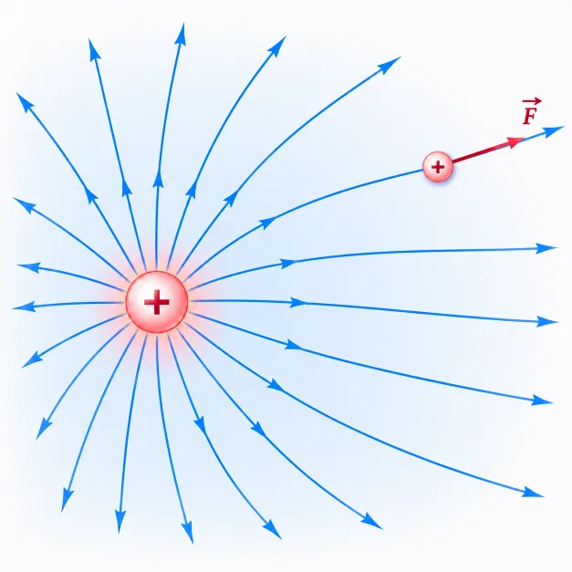
This illustration shows a positive source charge creating an electric field in the surrounding space. The blue field lines point outward, showing the direction a positive test charge would be pushed at each location. A small positive test charge placed on one field line experiences a force tangent to that field line, in the same direction as the electric field. The image helps students understand that the field already exists before the test charge is introduced; the test charge simply reveals the field by responding to it.
Learning Pathway in Electricity and Magnetism
Electricity and Magnetism
Introduces the overarching academic domain governing electric and magnetic phenomena, spanning static charges, dynamic currents, magnetic induction, and Maxwellian systems.
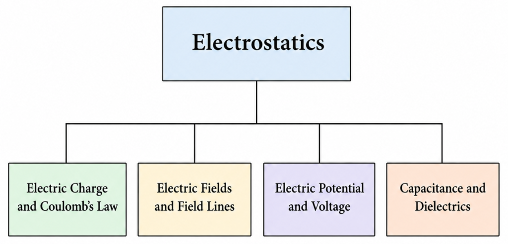
Electrostatics Parent Hub
Provides the primary conceptual umbrella, focusing on static charge systems in structural equilibrium and their associated field and potential distributions.
Electric Charge and Coulomb’s Law
Establishes the initial quantitative entry point, defining charge quantization, tribal interactions, and the primary inverse-square force equations.
Electric Fields and Field Lines
Advances past dual-source force tracking to map space as a continuous vector field modified by isolated source charges.
Electric Potential and Voltage
Transforms the structural analysis from vector forces to conservative scalar landscapes, defining electrical pressure as potential energy per unit charge.
Capacitance and Dielectrics
Applies field mappings and potential integrations to material polarization boundaries, physical hardware capacitors, and volumetric energy density metrics.
The Core Physical Idea
Field Lines Around Positive and Negative Charges
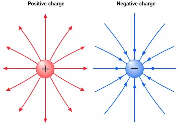
This illustration compares the electric field-line patterns around a positive charge and a negative charge. Around the positive charge, the arrows point outward because a positive test charge would be pushed away. Around the negative charge, the arrows point inward because a positive test charge would be pulled toward it. The image helps students understand that electric field direction follows the force direction on a positive test charge.
Uniform Electric Field Between Parallel Plates
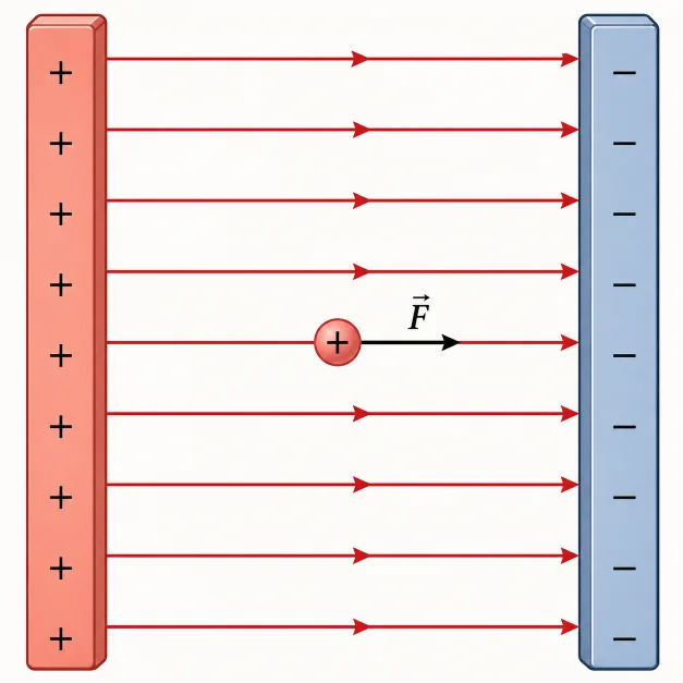
This illustration shows a uniform electric field between two oppositely charged parallel plates. The field lines are straight, evenly spaced, and directed from the positive plate toward the negative plate. A positive test charge placed between the plates experiences a force in the same direction as the electric field. The image helps students see why the electric field between large parallel plates is often treated as nearly constant in both strength and direction.
How a Test Charge Responds to an Electric Field
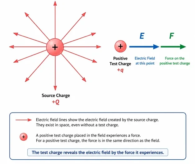
This illustration shows how a positive test charge responds when placed in an electric field. The electric field already exists in the space around the source charge, even before the test charge is introduced. When the positive test charge is placed at a point in the field, it experiences a force in the same direction as the electric field. This helps students understand that a test charge does not create the field being studied; it reveals the field by responding to it.
The Primary Pillar to Remember
An electric field is a continuous vector modification of space generated by charge distributions; field lines provide the geometric shorthand mapping its local force direction and magnitude.
Visualizing the Field Landscape
Picture the Source Node
Start with the source configuration that modifies the region. A positive source charge pushes field lines radially outward, while a negative source maps inward vectors.
Imagine the Unit Test Charge
Visualize a tiny, positive placeholder particle. The path it travels under local electrical strain defines the definitive vector direction arrow of the field at that coordinate.
Evaluate Volumetric Spacing
Look at the geometric line density. Where vector lines crowd closely, field strength is highly intense; where they branch apart, force magnitudes drop rapidly.
Reject the Wire Analogy
Field lines are structural map indicators, not physical paths or rails. A moving charge with initial velocity will curve dynamically across lines, rather than tracking them rigidly.
Key Equations and Physical Interpretations
Physical Meaning of E
The vector field quantity E reveals the specific force intensity that each single coulomb of positive charge experiences at that coordinate point, measured in Newtons per Coulomb (N/C).
Vector Directionality Symmetries
Because the field is a vector, it possesses distinct spatial coordinates. Arrows are mathematical necessities when mapping it across multi-dimensional layouts.
Inverse-Square Field Thinning
For standalone point nodes, field intensity degrades matching an inverse-square relationship (1/r²). Doubling spatial distance drops regional field strength to exactly 25% of baseline.
From Formula to Meaning
Advanced Mathematical Rigor: Continuous Field Integrals and Flux Dynamics
Technical Case Studies: Electric Fields in Applied Technology
Micro-Fluidic Trajectory Control: Inkjet Systems
Industrial printing printheads rely on steady electric fields to place microscopic ink droplets at precise geometric coordinates. Droplets exiting the nozzle receive a uniform, controlled electrostatic charge profile. They are then projected past a pair of deflection plates that maintain a strong, uniform electric field vector ($\mathbf{E} = \mathbf{F}/q$). By modifying plate voltage on a microsecond scale, engineers adjust the local field vector to deflect ink paths with sub-millimeter precision.
Biomedical Size Sorting: Gel Electrophoresis
Molecular laboratories apply uniform linear electric fields through porous gel matrices to separate macromolecular fragments like DNA. Because DNA backbones carry net negative charges, applying a stable electric field vector exerts an explicit mechanical force pulling the molecules toward the positive anode block. Shorter strands maneuver through the dense gel network faster than long chains, sorting the biological fragments perfectly by size.
Evolution of Field Theory: History, Micro-Limits, and Frontiers
Historical Epochs: The Transition to Continuous Spatial Topologies
Contemporary Challenges: Managing Field Breakdown in Nano-Scale Gates
Future Technological Horizons: High-Speed Optoelectronic Metamaterials
Numerical Problems and Solutions
-
A positive test charge of 2.0 × 10⁻⁹ C experiences a mechanical force of 1.0 × 10⁻³ N inside a localized electric field. Find the field strength.Solution: Apply the normalized base formula:$$E = \frac{F}{q} \Rightarrow E = \frac{1.0 \times 10^{-3}\text{ N}}{2.0 \times 10^{-6}\text{ C}} = 500\text{ N/C}$$Interpretation: The field intensity is exactly 500 N/C, directing force along the vector baseline independent of the test charge.
-
Determine the electric field magnitude at a spatial distance of 0.30 m from an isolated point charge of +4.0 μC.Solution: Deploy the radial inverse-square model:$$E = k_e \frac{|Q|}{r^2}$$ $$E = (8.99 \times 10^9) \frac{4.0 \times 10^{-6}\text{ C}}{(0.30\text{ m})^2} = \frac{35\,960}{0.09} \approx 4.0 \times 10^5\text{ N/C}$$Interpretation: The positive source creates a field intensity of 400,000 N/C pointing radially outward at that 0.30 m boundary coordinate.
-
A negative charge of -3.0 × 10⁻⁶ C is placed inside a uniform electric field carrying a value of 800 N/C. Calculate the resulting force vector magnitude.Solution: Isolate force using the field equation:$$F = |q|E \Rightarrow F = (3.0 \times 10^{-6}\text{ C})(800\text{ N/C}) = 2.4 \times 10^{-3}\text{ N}$$Interpretation: The force measures 2.4 × 10⁻³ N. Because the charge matches a negative sign value, the force vector acts directly opposite to the field direction lines.
-
Two identical positive point charges are positioned symmetrically on the horizontal axis around a center node. Determine the net electric field vector at the exact midpoint.Solution: The field generated by the left charge points to the right at the midpoint, while the field from the right charge points to the left with matching magnitude. Applying the principle of superposition requires evaluating their vector sum:$$\mathbf{E}_{\text{net}} = \mathbf{E}_{\text{left}} + \mathbf{E}_{\text{right}}$$ $$\mathbf{E}_{\text{net}} = E\hat{\mathbf{i}} + (-E\hat{\mathbf{i}}) = 0$$Interpretation: Geometric symmetry cancels the field vectors completely; the net field value at the midpoint is exactly zero.
Common Conceptual Misconceptions
The Physical Wire Illusion
Misconception: Field lines are real physical cords or wires running through the vacuum of space.
Reality: Field lines are abstract visual tools. The underlying electric field forms a continuous vector field that exists natively at every coordinate point in the spatial domain.
Source Modification Error
Misconception: Altering the size of the test charge changes the intensity value of the background field.
Reality: The field maps the background condition of space set by the source charge. Changing the test charge scales the force vector proportionally, keeping the field ratio fixed.
Applications of Electric Fields
Static Electricity Phenomena
A charged balloon, comb, or plastic ruler creates an electric field around itself. Nearby lightweight objects can respond to that field.
Capacitor Arrays
Capacitors store separated charge and create electric fields between their plates. This idea becomes important in energy storage and circuits.
Touchscreen Arrays
Many touch-sensitive devices depend on electric fields and changes in charge distribution near a surface.
Controlled Particle Beams
Charged particles can be accelerated or deflected by electric fields, a principle used in scientific instruments and particle physics experiments.
Real-World Illustration
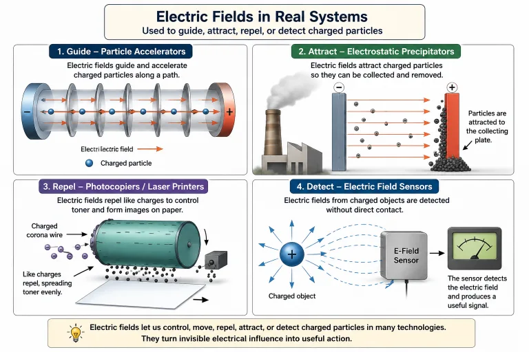
This illustration shows how electric fields move beyond classroom diagrams into practical technologies. Electric fields can guide charged particles in accelerators, attract particles in electrostatic precipitators, help control toner in printers, and allow sensors to detect charged objects without direct contact. The image helps students understand that an electric field is not just an invisible idea on paper; it can be used to control, move, collect, or detect charge in real systems.
Bridge to University Thinking
Quick Interactive Check
Show answer
Suggested answer: The field lines point away from the positive charge, because a positive test charge would be repelled outward.
Show answer
Suggested answer: The field lines point toward the negative charge, because a positive test charge would be attracted inward.
Show answer
Suggested answer: Closer field lines indicate a stronger electric field. Wider spacing indicates a weaker field.
Show answer
Suggested answer: No. A negative charge experiences a force opposite to the electric field direction.
Review Questions and Answers
- What is an electric field?Answer: An electric field is a region of influence created by electric charge. It describes the electric force per unit positive test charge at each point in space.
- What is the formula defining electric field?Answer: The electric field is defined by $\mathbf{E} = \frac{\mathbf{F}}{q}$, where $\mathbf{F}$ is the force on a test charge $q$.
- What is the unit of electric field?Answer: The unit of electric field is newtons per coulomb, written as N/C.
- Which way do electric field lines point around a positive charge?Answer: They point away from a positive charge.
- Which way do electric field lines point around a negative charge?Answer: They point toward a negative charge.
- What does closer spacing of field lines indicate?Answer: Closer spacing indicates a stronger electric field.
- Do field lines represent actual physical strings in space?Answer: No. Field lines are visual representations of the electric field, not physical objects.
- What direction is the electric field defined to have?Answer: The electric field direction is defined as the direction of the force on a small positive test charge.
Thought-Provoking Questions and Answers
- Why is the field idea more powerful than simply talking about forces between pairs of charges?Suggested answer: The field idea allows us to describe the condition of space around charges. Instead of calculating only one interaction at a time, we can describe what any charge would experience at any location.
- Why might students find invisible fields difficult to accept at first?Suggested answer: Fields are not visible objects, so students may look for something physical like a thread, stream, or wire. The challenge is to understand fields as measurable physical influence, even when the field itself is not directly seen.
- Why do field lines never cross in a normal electric field diagram?Suggested answer: If two field lines crossed, the field at that crossing point would have two directions at once. But the electric field at a single point has only one unique direction.
- How does the electric field idea prepare students for voltage?Suggested answer: Electric field focuses on force per unit charge, while voltage focuses on energy per unit charge. Understanding the field gives students a physical picture before they move into energy and potential difference.
- Why is it useful to think of electric field as a property of space rather than only a property of a charge?Suggested answer: It helps students see that a charge changes the surrounding space. Another charge placed there responds to the field already present at that location.
Summary
Authoritative External References
- OpenStax University Physics Vol 2: The Electric Field — Peer-reviewed academic documentation detailing spatial vector field mappings and continuous point-source calculus.
- OpenStax University Physics Vol 2: Electric Field Lines — Comprehensive reference for geometric field mappings and flux tracking conventions.
- Physics LibreTexts: Electric Field Lines — Core educational index highlighting continuous field distributions and boundary conditions.
- The Feynman Lectures on Physics, Vol. II, Chapter 1: Electromagnetism — Caltech’s premier lectures on physical theory, providing insights into electromagnetic field properties.