Prepare for University Studies & Career Advancement
Ampère’s Law: Symmetry and Magnetic Fields
Ampère’s law represents one of the most mathematically elegant and operationally efficient pillars of classical magnetostatics. It establishes a direct scalar relationship between the directional circulation of a magnetic field along a closed path and the net macro-scale electrical current piercing the interior surface bounded by that path. Instead of evaluating complex, three-dimensional vector integrations across custom geometries piece-by-piece—as mandated by the Biot–Savart law—Ampère’s circuital framework exploits natural geometric symmetries to evaluate magnetic flux maps cleanly.
The core utility of this framework rests entirely on spatial uniformity. When a steady electrical current configuration possesses a highly regular coordinate distribution, its surrounding magnetic flux lines mimic that symmetry profile. A long, straight line conductor establishes concentric, circular field tracks; an extended cylindrical solenoid generates a homogeneous axial field landscape within its core; and a closed toroid ring confines its total flux lines entirely inside a ring-shaped geometric matrix. Ampère’s law provides students and engineers with the mathematical tools required to parse these highly regular field structures systematically.
For university-level physics students, mastering Ampère’s law requires moving past basic algebraic plug-and-chug methods to cultivate an intuitive grasp of vector field configurations. It demands an advanced capability to recognize hidden geometric symmetries, select custom closed integration boundaries known as Ampèrian loops, account for signed current distributions, and physically map vector line distributions. Cultivating these analytical habits is an essential prerequisite before transitioning to time-dependent fields and advanced Maxwellian electrodynamics.
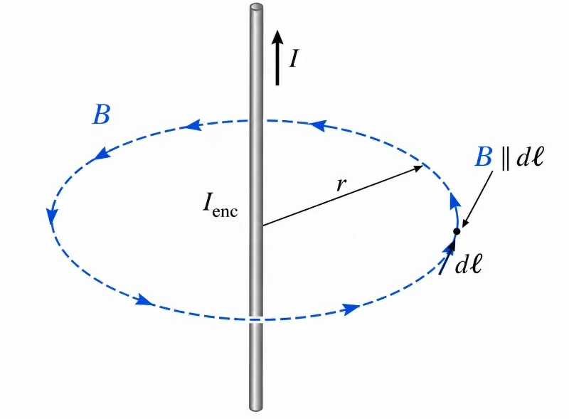
For a long straight wire, the magnetic field is tangent to a circular Amperian loop, making Ampère’s law simple to apply.
This illustration shows Amp`re’s law applied to a long straight wire carrying current upward. A dashed circular Amp`rian loop surrounds the wire and is shown clearly in front of the conductor, with magnetic field arrows tangent to the loop. The radius r marks the distance from the wire to the loop, while Ienc identifies the current enclosed by the Amp`rian path. The small loop element dℓ is shown in the same direction as the magnetic field B, helping students see why B is parallel to dℓ along the circular path. The diagram supports the key idea that symmetry allows the line integral in Amp`re’s law to simplify for a long straight current-carrying wire.
Magnetic Fields Learning Pathway
This subpage belongs to the Magnetostatics module within the broader Electricity and Magnetism curriculum. It sits directly between the element-based Biot–Savart law and the macroscopic evaluation of dipole distributions in matter, demonstrating how integral calculus simplifies calculation tasks for symmetrical systems.
Provides the global parent context for understanding charge distributions, vector field equations, electric circuits, induction, and Maxwellian wave mechanics.
Introduces how steady, time-independent currents configure local space to generate constant magnetic fields and establish forces across material systems.
Evaluates magnetic fields by executing brute-force differential integrations along arbitrary, non-symmetrical current-carrying line contours.
Ampère’s Circuital Law
Deploys closed line integrals and spatial symmetry profiles to extract exact magnetic field values for regular, uniform current distributions without direct integration.
Analyzes atomic magnetic moments, domain boundaries, magnetization vectors, and how materials alter ambient flux paths.
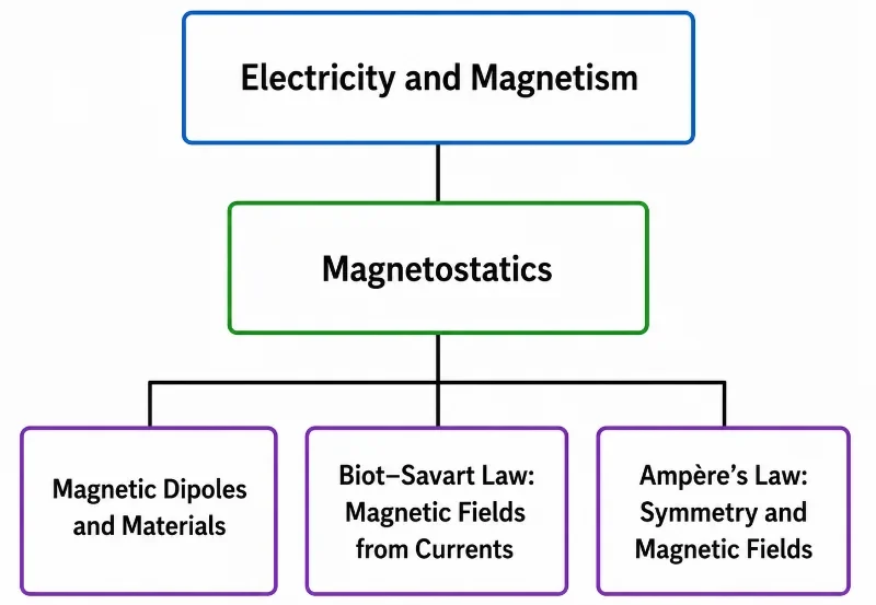
This tree chart shows the Magnetostatics cluster within Electricity and Magnetism, with its three child pages rearranged in a new order.
This hierarchy chart shows Magnetostatics as a highlighted sub-cluster within the wider Electricity and Magnetism section. The top node is Electricity and Magnetism, followed by the highlighted Magnetostatics hub. Below it are three related learning pages: Amp`re’s Law: Symmetry and Magnetic Fields, Biot–Savart Law: Magnetic Fields from Currents, and Magnetic Dipoles and Materials. The chart helps students see that Magnetostatics connects magnetic-field calculation, current geometry, symmetry, and material response within one coherent learning pathway.
The Core Mathematical Formulation
Ampère’s circuital law states that the closed line integral of the magnetic flux density vector taken around an arbitrary closed path matches the net electrical free current threading the enclosed surface area, scaled by the vacuum permeability constant. In time-independent systems, this relation is expressed in its definitive macroscopic integral form:
The left side evaluates the magnetic circulation, measuring how closely the field vectors align with the chosen integration path. The right side registers the total free current piercing the cross-sectional boundary sheet. Applying Stokes’ theorem transforms this relationship into its equivalent differential Maxwell equation:
$$\nabla \times \mathbf{B} = \mu_0 \mathbf{J}$$
This differential expression shows that the local curl of a magnetic field is driven exclusively by the local electrical current density vector at that point. It is critical to recognize that while Ampère’s law is fundamentally true for all steady current systems, it functions as a practical tool for calculating fields if and only if the current distribution possesses a high degree of spatial symmetry. Without sufficient symmetry, the integral remains true but cannot be simplified to isolate the field parameter algebraically.
Deconstructing the Integral Components
To safely translate the integral equation into algebraic relations without triggering parsing errors, each individual variable block must be precisely defined:
Closed Path Operator (∮)
Mandates that the line integration must execute continuously around a completely unbroken, closed path termed an Ampèrian loop.
Magnetic Flux Density (B)
Defines the localized magnetic field vector present at each differential step along the chosen Ampèrian integration line.
Differential Displacement (dℓ)
Represents an infinitesimal vector step taken along the boundary path, pointing tangent to the direction of integration travel.
Vector Dot Product (B · dℓ)
Extracts exclusively the parallel projection of the magnetic field vector along the integration line, dropping any perpendicular components.
Enclosed Net Current (Ienc)
Tracks the algebraic sum of all free electrical currents piercing the continuous surface area bounded by the outer path.
Vacuum Permeability (μ0)
Establishes the fundamental magnetic scaling constant in a vacuum, holding a value of exactly 4π × 10-7 T·m/A.
The Physical Intuition of Magnetic Circulation
While the term “magnetic circulation” may sound highly abstract, it describes a very concrete geometric behavior. Imagine tracking a closed geometric loop while measuring how closely the surrounding magnetic field lines point along your direction of travel. If the field lines loop tightly along your path, the dot product adds up constructively, resulting in a large circulation value. If the field vectors run perpendicular to your path, or if they lack a clear direction relative to your loop, the net circulation cancels out to zero.
Ampère’s law asserts that this magnetic circulation can only exist if there is a net electrical current threading through the center of the loop. If no current pieces the enclosed surface, the net circulation around that loop is identically zero, even if strong magnetic fields are present nearby. This topological property is what makes the law incredibly effective for analyzing wires, solenoids, and toroids.
Strategic Selection of Ampèrian Loops
An Ampèrian loop is a purely mathematical construct; it does not correspond to a physical wire or boundary. Selecting an appropriate loop path requires matching the inherent coordinate symmetry of the target field. A strategically selected loop ensures that the magnetic field magnitude is either completely constant and parallel along segments of the path—allowing the field parameter to be pulled out of the integral—or perfectly perpendicular to the path, reducing that segment’s contribution to zero.
For an infinite straight line current, a circular path centered on the wire axis is ideal because the field lines match the circle’s curvature, keeping the field magnitude constant along the entire path. For an extended cylindrical solenoid, a rectangular path is chosen instead; one side sits inside the uniform interior core field, while the other sides either run perpendicular to the flux paths or sit outside where the ideal field drops to zero.
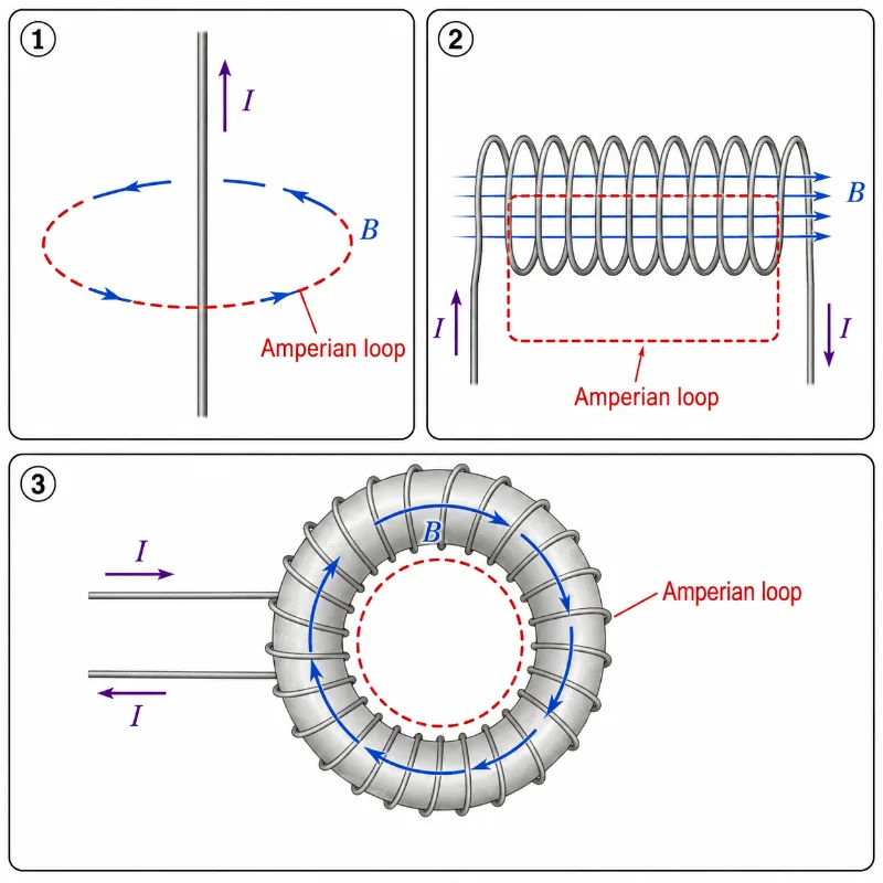
Ampère’s law becomes easiest to use when the Amperian loop matches the symmetry of the magnetic field.
This illustration compares three common choices of Amperian loop used with Amp`re’s law. A circular loop is shown around a straight current-carrying wire, matching the circular magnetic field pattern around the wire. A rectangular loop is shown through a solenoid, where the magnetic field is strong and nearly uniform inside the coil. A circular loop is also shown inside a toroid, where the magnetic field follows the ring-shaped core. The picture helps students understand that Amp`re’s law is most useful when the chosen loop follows the symmetry of the magnetic field.
Symmetry Classifications and Dimensional Reductions
Isolating magnetic field values algebraically relies on four primary spatial coordinate symmetries:
Infinite Line Symmetry
Applies to long straight wires and coaxial paths. The field vectors map out as concentric circles centered on the axis, making a circular loop the optimal choice.
Translational Invariance
Occurs along the extended length of regular wires or tightly wound solenoids, ensuring that the field profile looks identical at any cross-sectional slice along that axis.
Cylindrical Symmetry
Governs thick conductors and multi-layer cables. The current distribution depends solely on radial distance from the center, allowing the field to be solved inside and outside the material.
Toroidal Uniformity
Bends a cylindrical solenoid axis into a closed ring coordinate system, confining the total flux lines into a circular path inside the core shell.
Evolution of Circuital Calculus: History, Challenges, and Frontiers
To understand the progression of magnetostatic equations from basic observations into an exact field theory, we must trace their history, engineering challenges, and future horizons.
Historical Epochs: From Ampère’s Observations to Maxwell’s Extension
Following Hans Christian Ørsted’s 1820 discovery that an active current deflected a compass needle, French physicist André-Marie Ampère began a brilliant series of experiments to mathematically formalize these forces. By 1826, Ampère published his circuital loop relation, which connected the mechanical circulation of magnetic forces directly to the enclosed current. James Clerk Maxwell later referred to Ampère as the “Newton of electricity” because of the precision of this formula. However, in the 1860s, Maxwell realized that Ampère’s law was mathematically incomplete for time-varying systems because taking the divergence of both sides violated charge conservation. To resolve this, Maxwell introduced the concept of displacement current (ε0 ∂ E / ∂ t), expanding the formula into the Ampère–Maxwell equation and linking electricity and magnetism into a unified electromagnetic wave theory.
Contemporary Engineering Challenges: As-Symmetric Flux Leakage and Non-Uniform Current Sheets
While calculating fields with Ampère’s law is simple across ideal, infinite geometries, real-world engineering devices have finite boundaries that break these ideal symmetries. In high-power transformers, industrial electromagnets, and electric motors, fields cannot remain perfectly confined. Engineers face flux leakage at the edges of solenoids and toroids, where field lines bow outward into non-uniform paths that can interfere with nearby electronics. Furthermore, in high-frequency circuits, the current sheet approximations break down due to the skin effect, which forces currents to crowd toward the outer boundaries of a conductor rather than flowing uniformly through its cross-section. These edge effects require designers to use advanced computational finite element analysis (FEA) rather than simple integral equations.
Future Technological Horizons: High-Field Fusion Plasmas and Spintronic Circuits
Today, the principles of circuital field mechanics are driving breakthroughs in zero-carbon energy and quantum computing. In advanced nuclear fusion tokamaks, researchers use intense helical current paths to create a closed, toroidal magnetic bottle that confines hyper-hot plasma. Modeling these complex, self-induced plasma currents relies on magnetohydrodynamic interpretations of Ampère’s law to prevent volatile instabilities from disrupting the plasma bottle. On a microscopic scale, the field of spintronics is replacing traditional copper data channels with sub-micron spin-polarized current streams. By controlling localized current densities at the nanoscale, engineers can manipulate spin-transfer torques to flip magnetic domains instantly, enabling ultra-dense, non-volatile memory architectures with near-zero power dissipation.
Field Distribution Outside an Infinite Straight Conductor
To compute the magnetic field around an infinite straight wire carrying a steady current I, choose a circular Ampèrian loop of radius r centered on and perpendicular to the wire axis. By cylindrical symmetry, the magnetic field magnitude B must be completely uniform at every point along the circular path, and its orientation must point tangent to the loop vector:
Because the field magnitude B is constant along the circular line, it can be factored completely outside the line integral:
$$B \oint d\ell = \mu_0 I$$
The closed path integration of the displacement vector around the circle evaluates directly to its geometric circumference (2πr):
$$B(2\pi r) = \mu_0 I$$
Solving this relation for the field parameter B yields the classical line conductor expression:
$$B = \frac{\mu_0 I}{2\pi r}$$
This matches the result derived from the Biot–Savart law, but Ampère’s law reaches it more efficiently by exploiting the system’s geometric symmetry.
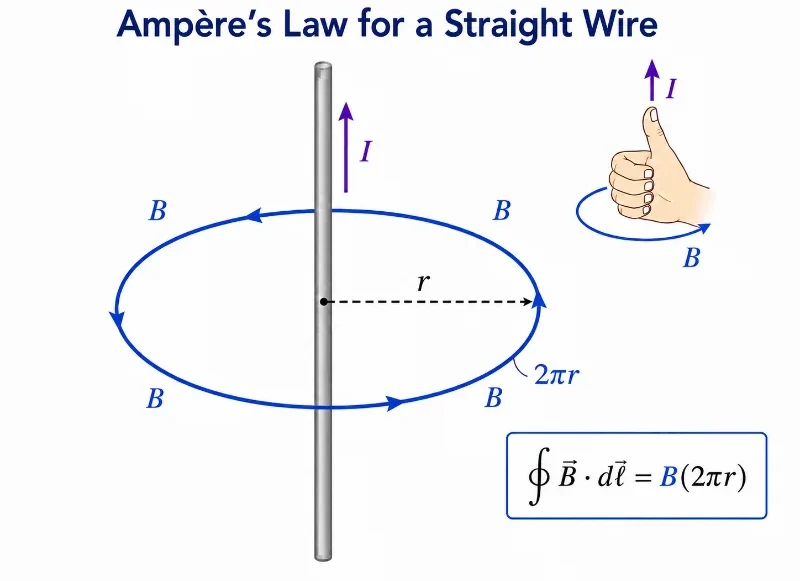
For a long straight wire, a circular Amperian loop matches the symmetry of the magnetic field, so the line integral simplifies to B(2πr).
This illustration shows how Amp`re’s law is applied to a long straight current-carrying wire. The current I flows upward through the wire, while the magnetic field B follows a circular path around it. The radius r marks the distance from the wire to the Amperian loop, and the label 2πr represents the circumference of that circular path. Because the magnetic field is tangent to the loop and has the same magnitude along the symmetric path, the line integral around the loop simplifies to B(2πr). The right-hand-rule cue helps students connect the upward current direction with the circular magnetic field direction.
Field Distribution Within an Ideal Solenoid Core
A solenoid consists of a long wire wound into a tight helical cylinder. When a steady current flows through its loops, the individual field contributions combine constructively along the central axis, establishing a strong, uniform magnetic field inside. For an ideal, infinitely long solenoid, the exterior magnetic field drops to zero.
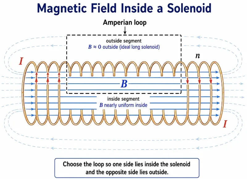
To evaluate an ideal solenoid containing n turns per meter carrying a current I, construct a rectangular Ampèrian loop passing partly inside and partly outside the core. The line integral splits into four distinct linear segments:
The segments running perpendicular through the solenoid walls contribute zero because the dot product vanishes ($\mathbf{B} \perp d\boldsymbol{\ell}$). The exterior segment also contributes zero because the ideal outside field is negligible. This leaves only the interior segment of length L, where the field runs perfectly parallel to the integration path:
$$B \cdot L = \mu_0 I_{\text{enc}}$$
Because the rectangular loop encloses a total of n·L individual wire turns, the net enclosed current equals Ienc = n L I. Substituting this value into the equation yields:
$$B \cdot L = \mu_0 (n L I) \Rightarrow B = \mu_0 n I$$
This fundamental formula dictates the operating limits of heavy electromagnets, industrial relays, and high-precision laboratory field coils.
A correct rectangular Amperian loop for a long solenoid has one long side inside the solenoid, where the magnetic field is strong and nearly uniform, and the opposite long side outside, where the field is negligible in the ideal case.
Field Distribution Within a Toroidal Core
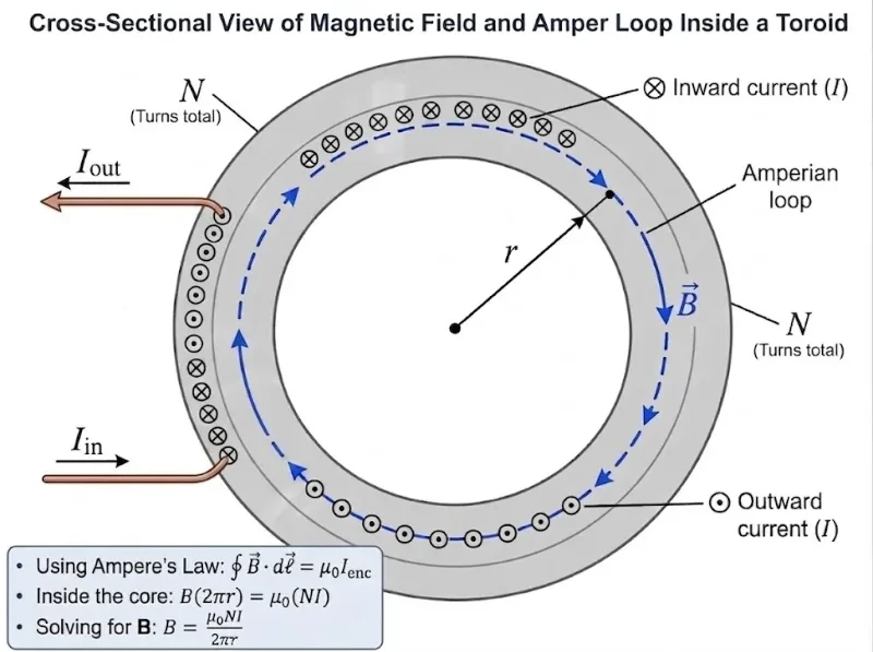
A toroid is essentially a linear solenoid bent into a closed circular ring, anchoring all magnetic flux lines entirely within its interior core. To calculate the field profile inside a toroid containing a total of N turns, implement a circular Ampèrian loop of radius r inside the core shell. Cylindrical symmetry ensures that the field magnitude is uniform along this circular path:
Because the circular integration line threads through every single loop turn on the inner wall, the net enclosed current matches the total number of turns multiplied by the current (Ienc = N I). Substituting this gives:
$$B(2\pi r) = \mu_0 N I \Rightarrow B = \frac{\mu_0 N I}{2\pi r}$$
This expression resembles the straight-wire result, but the field can be scaled upward by increasing the total number of turns N, allowing engineers to guide magnetic fields efficiently within transformers and inductor cores.
A toroid is best analysed using a circular Amperian loop inside the core, where the magnetic field follows the ring-shaped path and the loop encloses multiple current turns.
This cross-sectional illustration shows how Amp`re’s law is applied to a toroid. The toroidal core is shown as a ring, with current directions represented by dots and crosses to indicate current coming out of or going into the page. A dashed circular Amperian loop lies inside the core, following the same circular path as the magnetic field B. The radius r marks the distance from the centre of the toroid to the chosen Amperian loop. The diagram helps students see why the enclosed current is related to the total number of turns N and why the magnetic field inside the toroid is guided around the core rather than spreading outward like the field of a straight wire.
The Algebraic Sign Framework of Enclosed Currents
The current parameter Ienc measures the net algebraic sum of all free currents piercing the surface bounded by the Ampèrian loop. Currents traveling in opposite directions through this enclosed area must be tracked with opposite algebraic signs, preventing basic calculation errors.
To determine the correct mathematical sign systematically, use the Right-Hand Rule for Enclosed Currents: curl the fingers of your right hand along the chosen directional heading of the Ampèrian loop integration path. Your extended right thumb then establishes the positive vector heading. Any current vector pointing in your thumb’s direction adds as a positive current, while any current traveling opposite to your thumb subtracts as a negative current.
Students must remember that nearby electrical currents only alter the circulation integral if they actively pierce the bounding area of the loop. A wire placed outside the loop boundaries contributes nothing to the net enclosed current value.
Comparing Integral and Differential Calculi
While the Biot–Savart law and Ampère’s law both calculate magnetic field fields generated by steady electrical currents, their analytical application strategies differ completely:
The Biot–Savart Integral Law
Builds up fields by summing individual differential contributions from current line elements. It serves as the primary tool for computing fields around finite wires, broken loops, arcs, and arbitrary, non-symmetrical current paths.
Ampère’s Circuital Law
Binds the field circulation along a path directly to the total enclosed free current. It is incredibly efficient for solving highly symmetric current layouts, bypassing difficult multi-dimensional vector integration completely.
The Optimal Design Choice
Implement Ampère’s circuital integrals when high spatial symmetry allows the field parameter to be factored out cleanly. Use the Biot–Savart differential law when the system’s geometric profile breaks coordinate uniformity.
Industrial Applications: The Mechanics of Symmetrical Fields
Symmetrical field calculation forms the foundation of modern high-power transmission systems and heavy industrial machinery:
High-Voltage Power Distribution
Ampère’s law allows power grid engineers to model and map magnetic flux distributions around high-capacity industrial cables and multi-conductor lines without executing complex integrations.
Commercial Electromagnetic Solenoids
Solenoid core fields provide the mechanical pressure driving heavy-duty industrial relays, hydraulic control valves, automated actuators, and high-capacity laboratory field chokes.
High-Efficiency Toroidal Inductors
Toroidal cores are vital components in high-frequency power supplies, signal transformers, and noise filters because their closed circular geometry confines magnetic flux fields inside the ring core.
Concentric Coaxial Cable Balancing
Coaxial layouts utilize equal and opposite current paths across their inner and outer conductors. Ampère’s law proves that the exterior magnetic field drops to zero, shielding sensitive signals from interference.
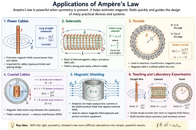
Ampère’s law helps estimate magnetic fields in symmetric current systems such as straight conductors, solenoids, toroids, coaxial cables, shielding structures, and laboratory setups.
This infographic shows how Amp`re’s law is used in physics and engineering whenever current systems have useful symmetry. It illustrates magnetic fields around power cables, nearly uniform fields inside solenoids, guided fields inside toroids, field cancellation in coaxial cables, magnetic-field control through shielding, and simple laboratory experiments using straight wires, solenoids, and toroids. The picture helps students see why Amp`re’s law is powerful: with the right symmetry, difficult magnetic-field calculations can become simpler and more physically intuitive.
Quick Check: Meaning of Ampère’s Law
Quick Check: Meaning of Ampère’s Law
1. What does Amp`re’s law relate?
Amp`re’s law relates the circulation of the magnetic field around a closed path to the net current passing through the surface enclosed by that path.
2. What is an Amperian loop?
An Amperian loop is a closed path chosen for applying Amp`re’s law. A good loop matches the symmetry of the magnetic field.
3. Why is symmetry important when using Amp`re’s law?
Symmetry can make the magnetic field constant along a path or perpendicular to parts of the path, allowing the line integral to become simple.
4. Does every nearby current count as enclosed current?
No. Only the net current passing through the surface bounded by the Amperian loop counts as Ienc.
Quick Check: Symmetry and Field Direction
Quick Check: Symmetry and Field Direction
1. What Amperian loop is best for a long straight wire?
A circular loop centred on the wire is best because the magnetic field is tangent to the loop and has the same magnitude everywhere on it.
2. What is the magnetic field direction around a long straight wire?
The magnetic field circles around the wire. Its direction is found by pointing the right thumb along the conventional current and curling the fingers.
3. What happens to the magnetic field around a wire if the current is reversed?
The magnetic field direction reverses, although the field lines still form circles around the wire.
Numerical Practice
Numerical Practice: Amp`re’s Law
1. A long straight wire carries 10 A. Find the magnetic field 0.25 m from the wire.
Use B = μ0I / (2πr). Substituting gives B = (4π × 10-7)(10) / (2π · 0.25) = 8.0 × 10⁻⁶ T.
2. A long solenoid has 1500 turns/m and carries 2.0 A. Estimate the magnetic field inside.
Use B = μ0nI. Substituting gives B = (4π × 10-7)(1500)(2.0) ≈ 3.77 × 10⁻³ T.
3. A toroid has 500 turns, current 1.2 A, and radius 0.15 m. Find the magnetic field inside the toroid at that radius.
Use B = μ0NI / (2πr). Substituting gives B = (4π × 10-7)(500)(1.2) / (2π · 0.15) = 8.0 × 10⁻⁴ T.
4. An Amperian loop encloses currents of 6.0 A, 2.0 A, and -3.0 A. What is the net enclosed current?
Add the currents algebraically: Ienc = 6.0 + 2.0 – 3.0 = 5.0 A.
Review Questions and Answers
Review Questions: Amp`re’s Law
1. State Amp`re’s law for magnetostatics.
The magnetostatic form is ∮ B · dℓ = μ0Ienc.
2. Why is Amp`re’s law especially useful for symmetric current distributions?
Symmetry can make B constant in magnitude and parallel to the path, allowing the line integral to simplify into a product such as B(2πr).
3. What is the magnetic field around a long straight wire?
The field magnitude is B = μ0I / (2πr), and the field lines form circles around the wire.
4. What is the magnetic field inside an ideal long solenoid?
For an ideal long solenoid, B = μ0nI, where n is the number of turns per metre.
5. What is the difference between Amp`re’s law and the Biot–Savart law?
The Biot–Savart law builds the field by adding contributions from current elements. Amp`re’s law uses magnetic circulation and enclosed current, and is most useful when symmetry is strong.
Thought-Provoking Questions
Thought-Provoking Questions
1. Why does Amp`re’s law reward good geometric thinking?
Because the law becomes powerful only when the chosen loop fits the symmetry of the magnetic field. A good geometric choice can turn a difficult field calculation into a simple relationship.
2. Why is it not enough to say that a current is “near” an Amperian loop?
Amp`re’s law depends on current passing through the surface enclosed by the loop, not merely on current that is nearby. The idea of enclosed current is topological as well as spatial.
3. Why does a solenoid produce a strong field inside but a much weaker field outside?
Inside a long solenoid, the magnetic field contributions from many turns reinforce in the same direction. Outside, the contributions tend to spread out and partly cancel, making the external field much weaker in the ideal case.
4. Why does the full Amp`re–Maxwell law become necessary in electrodynamics?
When electric fields change with time, conduction current alone is not enough to describe magnetic-field behaviour consistently. Maxwell’s displacement-current term completes the law for time-varying fields.
Glossary
Ampère’s law: A physical law mapping magnetic circulation along a closed path directly to the net electrical free current enclosed by that path loop.
Amperian loop: An arbitrary closed mathematical integration line chosen to evaluate circuital magnetic fields.
Magnetic circulation: The closed line integral value of the magnetic flux density vector along a closed path loop.
Enclosed current: The net free electrical current actively piercing the internal surface area bounded by an Ampèrian path loop.
Line integral: A mathematical integration calculus operation that evaluates field component projections along a path.
Solenoid: A cylindrical wire coil loop distribution capable of generating highly uniform axial field lines within its core cavity.
Toroid: A closed ring-shaped inductive wire winding structure that contains its total generated magnetic flux completely within its core parameters.
Vacuum Permeability (μ0): The universal scalar constant anchoring magnetic field metrics within free space environments.
Symmetry: A regular dimensional mapping pattern that enables complex partial differential integrations to reduce to clean algebraic relations.
Ampère–Maxwell law: The comprehensive time-dependent electrodynamic expression that appends displacement current terms to basic circuital current inputs.
Ampère’s circuital law mathematically links the line integral circulation of a magnetic field along an arbitrary closed path directly to the net free electrical current threading through the enclosed surface area sheet. In steady-state time-independent environments, this relationship functions via the classical integral equation ∮ B · dℓ = μ0Ienc.
The structural power of this electrodynamic relation shows up when dealing with high spatial symmetry configurations. For infinite line conductors, thick cylindrical cables, extended solenoids, and closed toroidal rings, selecting an Ampèrian integration path that mirrors the coordinate field loops allows the magnetic field parameter to be pulled outside the integral, reducing a difficult calculation task to simple multiplication.
The most critical diagnostic lesson for university preparation is learning how to recognize symmetry fields, choose optimal integration loops, track signs via right-hand parameters, and map out flux contours. Bypassing unneeded direct integration steps lets engineers design stable magnetic components intuitively.
Furthermore, mastering this static relation establishes the necessary mathematical bridge before students transition to full time-varying electrodynamic phenomena, where the addition of Maxwell’s displacement current parameter accounts for changing electric flux paths and supports electromagnetic wave propagation.
Reflection Question
If Ampère’s circuital law functions as an ironclad physical truth across all steady-state environments, yet acts as an effective operational tool for field calculations only when high spatial symmetry exists, what does this duality demonstrate about the foundational interplay between geometry, mathematics, and physical insight?