
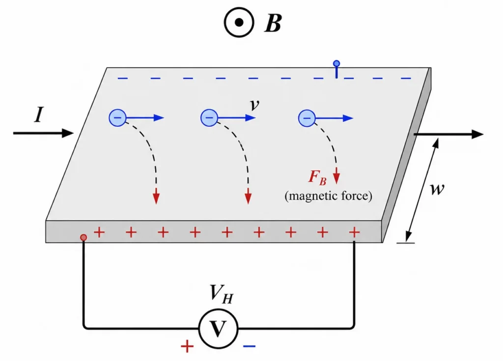
This diagram illustrates the Hall effect in a current-carrying strip placed in a magnetic field. As charge carriers move through the material, the magnetic field exerts a sideways force on them, causing negative charges to gather on one side and positive charge to appear on the opposite side. This separation of charge creates a measurable Hall voltage across the width of the strip. The picture helps students see how magnetic force, current flow, and charge separation combine to make magnetic field measurement possible.
Magnetic Fields Learning Pathway
Electricity and Magnetism Context
Provides the wider physics context for charge distributions, electric fields, electric circuits, magnetic fields, induction, and electromagnetic waves.Magnetic Fields Parent Hub
Introduces how magnetic fields exert forces, guide moving charges, interact with currents, and appear in measurement technologies.Magnetic Force on Moving Charges
Explains how a charged particle moving through a magnetic field experiences a sideways force depending on charge, speed, field strength, and angle.Magnetic Force on Current-Carrying Wires
Extends magnetic force from moving charges to a wire carrying current, explaining how magnetic fields can push conductors and produce motion.Motion of Charges in Magnetic Fields
Shows how magnetic force can produce circular, helical, or curved paths for charged particles moving through magnetic fields.Hall Effect and Magnetic Measurement
Explains how magnetic force separates charges inside a conductor or semiconductor, producing Hall voltage and enabling magnetic field sensors.The Core Physical Idea
Charge Separation in the Hall Effect
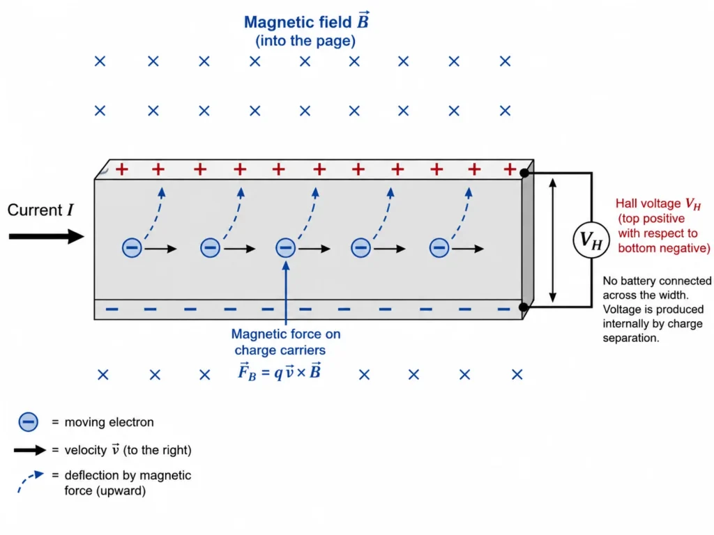
This illustration shows how the Hall effect produces a voltage across a current-carrying material. As charge carriers move along the strip, a magnetic field acting perpendicular to their motion pushes them sideways. This causes charge to build up on opposite sides of the strip, creating a Hall voltage across its width. The picture helps students see that the Hall voltage is not supplied by a battery across the strip, but is generated internally by magnetic-force-driven charge separation.
Direction of Hall Voltage for Different Charge Carriers
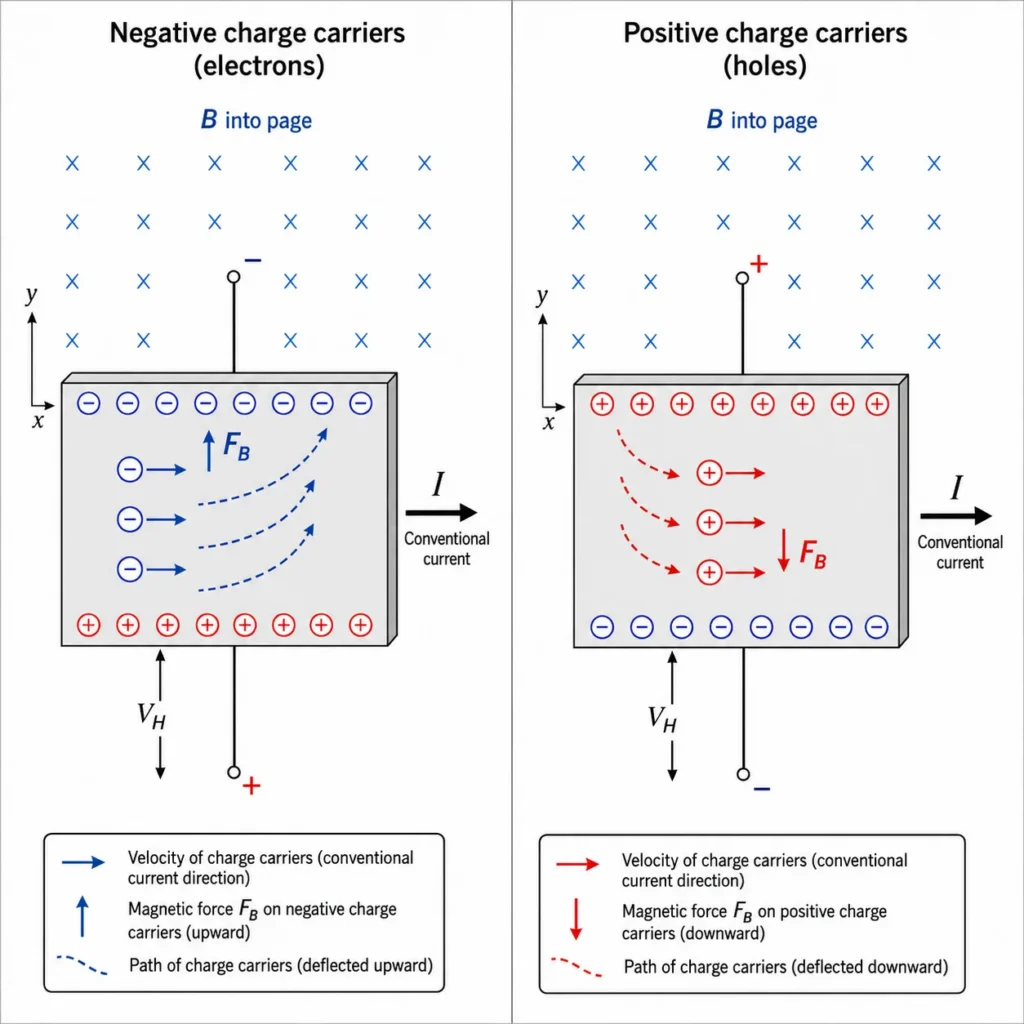
This illustration compares the Hall effect for two different kinds of charge carriers under the same current direction and magnetic field direction. In one case, negative charge carriers (electrons) are deflected sideways and produce one Hall voltage polarity. In the other case, positive charge carriers (holes) are deflected in the opposite way and produce the opposite Hall voltage polarity. The picture helps students see why the Hall effect is useful in material science: by observing the direction of the Hall voltage, we can infer whether a material conducts mainly through electrons or through positive holes.
Hall Sensor Measuring a Magnetic Field
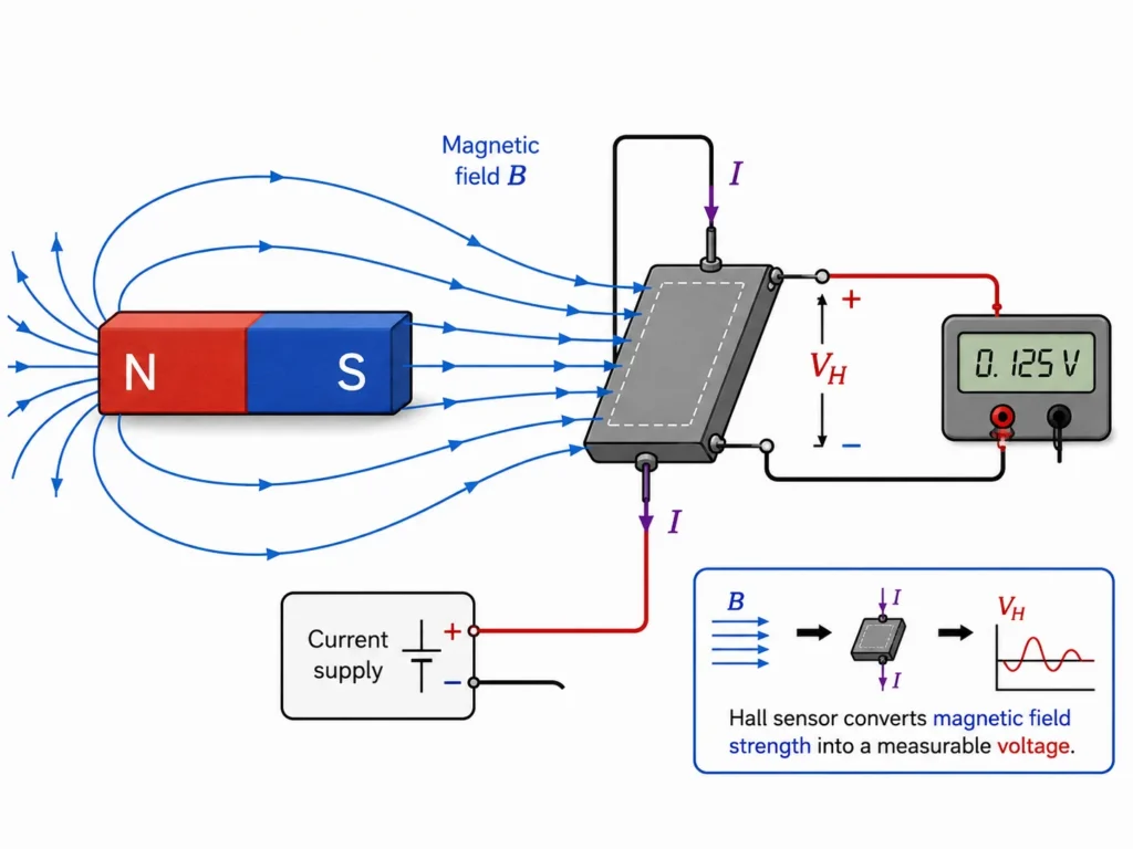
This illustration shows a Hall sensor placed near a magnet so that magnetic field lines pass through the sensor element. A current supply drives charge carriers through the sensor, and the magnetic field causes a Hall voltage to appear across the device. The output voltage is then measured electronically. The picture helps students see how the Hall effect is used in practice to detect magnetic fields and convert them into usable electrical signals.
How Hall Voltage Is Produced
Longitudinal Carrier Drift
An applied longitudinal voltage drives a steady drift of free charge carriers through the thin element, establishing the primary velocity vector required for magnetic interaction.Transverse Deflection Force
The perpendicular magnetic field exerts a continuous sideways force, driving the incoming charge carriers toward one cross-sectional wall.Boundary Charge Accumulation
As carriers accumulate on one edge, they form a polarized boundary layer that creates a steady transverse electric field across the material’s width.Dynamic Force Equilibrium
The transverse electric field intensifies until its electrostatic force perfectly balances the Lorentz magnetic force, forcing subsequent current streams to pass straight through without further deflection.The Core Principle to Remember
The Hall effect maps microscopic, sideways magnetic forces acting on moving charges into an easily amplified, macroscopic transverse voltage signal.
Key Equations and Material Parameter Analysis
Longitudinal Current (I)
Elevating current values increases carrier velocity vectors, maximizing cross-gap deflection forces and raising the final voltage output linearly.Magnetic Flux Density (B)
A more intense ambient magnetic field directly scales the sideways force, producing a larger boundary charge separation and a larger Hall voltage signal.Volumetric Carrier Density (n)
Materials with low carrier concentrations require a faster drift velocity to sustain a given current, which increases the required balancing field and produces a larger Hall voltage.Element Thickness (t)
Thinner semiconductor strips confine the current flow to a compressed volume, increasing local charge carrier densities to maximize the resulting voltage signal.From Formula to Meaning
Advanced Mathematical Rigor: The Tensor Conductivity Matrix
Worked Analytical Example
- Current (I) = 0.020 A
- Magnetic Flux Density (B) = 0.50 T
- Carrier Density (n) = 2.0 × 10²² m-3
- Elementary Charge (q) = 1.6 × 10⁻¹⁹ C
- Element Thickness (t) = 1.0 × 10⁻³ m
Worked Example Visual Representation
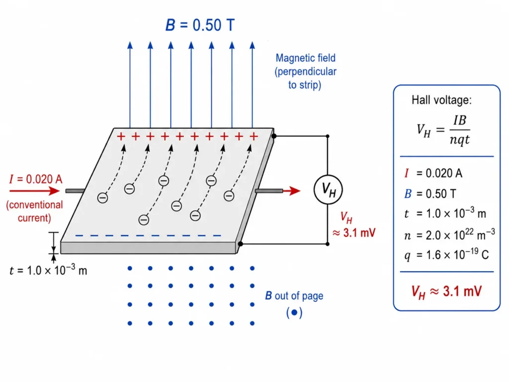
This illustration shows a worked example of Hall voltage production in a Hall sensor strip. A current of 0.020 A flows through the strip while a magnetic field of 0.50 T acts perpendicular to the material. Moving charge carriers are deflected sideways, producing charge separation and a small Hall voltage across the strip. Using the formula V_H = IB/(nqt), the Hall voltage is estimated to be about 3.1 mV. The picture helps students connect current, magnetic field strength, material thickness, carrier density, and Hall voltage in one clear calculation.
Common Conceptual Misconceptions
The Supply Voltage Confusion
Misconception: The Hall voltage signal is simply a fraction of the primary voltage driving current down the wire. Reality: The Hall voltage is a completely separate transverse potential difference. It acts completely perpendicular to the primary driving voltage circuit, generated entirely by internally separated charge distributions.The Identical Deflection Myth
Misconception: Because negative electrons and positive holes carry opposite signs, they are deflected toward opposite walls inside the sensor. Reality: They accumulate on the exact same boundary wall. Because a current of holes moving forward matches the vector force direction of electrons moving backward under cross-product rules, the magnetic force pushes both carrier types toward the same edge. The charge sign difference is revealed solely by the polarity of the resulting voltage.Real-World Engineering Frameworks
Automotive Speed Tracking
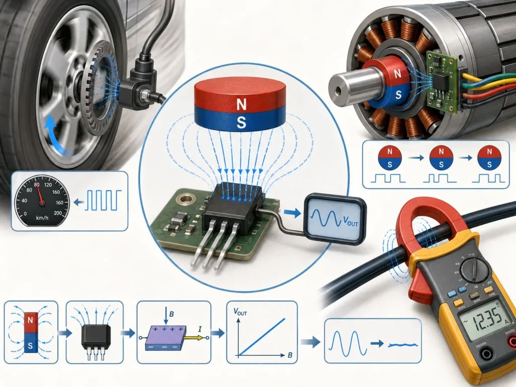
Anti-lock braking systems (ABS) place Hall sensors next to notched magnetic target wheels on rotating axles. As the wheel spins, the passing teeth fluctuate the local magnetic field, generating a pulsed Hall voltage that microchips translate into real-time wheel speed data.Brushless DC Commutation
Brushless motors use internal Hall-effect arrays to monitor the exact rotational position of the permanent magnet rotor, allowing onboard electronics to switch stator coils smoothly to maintain maximum torque.Non-Intrusive Current Monitoring
Professional current clamp meters utilize a high-permeability iron core to channel the circular magnetic field lines encircling a live wire directly into an integrated Hall sensor, measuring active currents safely without cutting the wire.Real-World Engineering Applications
Bridge to University Thinking
Quick Interactive Check
Quick Check: The Hall Effect and Magnetic Measurement
Test your grasp of solid-state transverse field dynamics using these conceptual checkpoints:
Review Questions and Answers
- What is the Hall effect?Answer: The Hall effect is the production of a steady transverse voltage difference across a current-carrying material exposed to an external perpendicular magnetic field.
- What causes the generation of a Hall voltage?Answer: Hall voltage is caused by the magnetic Lorentz force deflecting moving charge carriers sideways, producing a localized charge separation across the material’s width.
- State the scalar formula for the Hall voltage in a basic rectangular system.Answer: The potential is calculated via the relationship: VH = I B / (n q t).
- Why does the resulting Hall voltage depend linearly on the ambient magnetic flux density?Answer: A more intense magnetic field increases the transverse Lorentz force acting on the carriers, separating additional charge until a larger balancing voltage builds up across the gap.
- How can the Hall effect identify a material’s majority carrier type?Answer: Because the cross-product forces both positive and negative carriers toward the same edge, the absolute mathematical sign of the majority carrier dictates the electrical polarity of the resulting voltage signal.
- What does the Hall coefficient track?Answer: The Hall coefficient (RH = 1 / nq) tracks a material’s fundamental electronic configuration, matching carrier type signs and volumetric densities.
- What are some common industrial uses for Hall-effect hardware?Answer: Hall-effect hardware is used to map ambient magnetic field profiles, track anti-lock wheel braking speeds, monitor rotor positions inside brushless motors, and execute non-intrusive current measurements.
- What fundamental physical law underpins the Hall effect?Answer: The effect is built entirely on the magnetic component of the Lorentz force law, tracking point charge forces perpendicular to motion.
Thought-Provoking Questions and Answers
- Why does the Hall effect prove that electrical current is a physical stream of moving particles rather than an abstract fluid?Suggested answer: If current were a continuous, non-particulate fluid, an external magnetic field could not separate discrete charge carriers across a material’s width. The build-up of a measurable transverse voltage drop confirms that electrical current is a directed stream of individual moving particles that respond to cross-product forces.
- Why do electron and hole carriers migrate toward the exact same boundary wall under identical current and field configurations?Suggested answer: According to semiconductor physics, a forward current of positive holes matches the vector force direction of a reverse stream of negative electrons. Because the cross-product relationship flips signs twice (inverting both the charge carrier sign and its velocity vector direction), the resulting force vector points toward the exact same edge in both cases.
- How does the Hall effect connect electrostatics to magnetostatics inside solid-state materials?Suggested answer: The phenomenon acts as a direct mechanical bridge between both domains. The moving charge carriers are initially deflected sideways by a magnetostatic Lorentz force, which establishes an electrostatic potential gradient across the material that intensifies until its electric force perfectly balances the primary magnetic deflection.
Numerical Problems and Solutions
- A specialized semiconductor chip handles a current of 0.010 A inside a uniform 0.20 T magnetic field. The material carries a carrier density of 1.0 × 10²² m-3, a charge carrier footprint of 1.6 × 10⁻¹⁹ C, and an element thickness of 1.0 × 10⁻³ m. Calculate the resulting Hall voltage.Solution: Apply the scalar geometry ratio formula:$$V_H = \frac{IB}{nqt}$$ $$V_H = \frac{(0.010\text{ A})(0.20\text{ T})}{(1.0 \times 10^{22}\text{ m}^{-3})(1.6 \times 10^{-19}\text{ C})(1.0 \times 10^{-3}\text{ m})}$$ $$V_H = \frac{0.0020}{1.6} = 1.25 \times 10^{-3}\text{ V}$$Answer: The resulting Hall voltage drop measures exactly 1.25 mV.
- If an engineered Hall sensor’s voltage output doubles while the driving current and element thickness remain completely unchanged, what physical shift has occurred in the ambient magnetic field environment?Solution: Analyze the scaling relationships within the primary equation:$$V_H \propto B$$Answer: Because Hall voltage scales linearly with the magnetic flux density parameter, the ambient magnetic field must have exactly doubled in intensity.
- A transverse Hall potential of 2.0 mV is recorded across an industrial sensor strip handling a current of 0.020 A inside a 0.40 T magnetic field. If the carrier charge equals 1.6 × 10⁻¹⁹ C and the film thickness measures 2.0 × 10⁻³ m, calculate the material’s volumetric carrier density n.Solution: Rearrange the primary algebraic equation to isolate the carrier density parameter:$$n = \frac{IB}{V_H q t}$$ $$n = \frac{(0.020\text{ A})(0.40\text{ T})}{(2.0 \times 10^{-3}\text{ V})(1.6 \times 10^{-19}\text{ C})(2.0 \times 10^{-3}\text{ m})}$$ $$n = \frac{0.0080}{6.4 \times 10^{-25}} = 1.25 \times 10^{22}\text{ m}^{-3}$$Answer: The material’s intrinsic volumetric carrier density equals 1.25 × 10²² m-3.
- An automotive sensor block maintains a calibrated sensitivity parameter of 40 mV/T. Determine the absolute output voltage change expected when the system is exposed to an operating field shift of 0.15 T.Solution: Scale the field metrics by the baseline extraction coefficient:$$\Delta V = (\text{Sensitivity}) \cdot \Delta B$$ $$\Delta V = (40\text{ mV/T})(0.15\text{ T}) = 6.0\text{ mV}$$Answer: The expected output voltage change measures exactly 6.0 mV.
Evolution of Hall Anomalies: History, Micro-Limits, and Frontiers
Historical Epochs: From Classical Deflection to Quantum Hall Symmetries
Contemporary Engineering Challenges: Thermal Drift and Material Saturation
Future Horizons: Quantum Anomalous Hall Topologies and Spintronic Gates
Summary
Glossary
- Hall Effect
- The production of a sideways voltage across a current-carrying material placed in a magnetic field.
- Hall Voltage
- The voltage produced across a conductor or semiconductor due to sideways charge separation in a magnetic field.
- Hall Sensor
- A sensor that uses the Hall effect to detect or measure magnetic fields.
- Charge Carrier
- A mobile charged particle, such as an electron or hole, that carries electric current through a material.
- Carrier Density
- The number of mobile charge carriers per unit volume of material.
- Hall Coefficient
- A material property related to carrier density and charge carrier sign.
- Drift Velocity
- The average velocity of charge carriers moving through a material due to an electric field.
- Magnetic Field Strength
- The strength of a magnetic field, represented by B and measured in tesla.
- Contactless Measurement
- Measurement without direct mechanical contact, often using magnetic or optical sensing.
- Semiconductor
- A material whose electrical conductivity can be controlled and whose charge carriers may be electrons or holes.
Frequently Asked Questions
What is the Hall effect in simple terms?
The Hall effect is the creation of a small sideways voltage drop across a conductive strip when electrical current passes through it inside an external magnetic field.
Why does the Hall voltage appear?
It appears because the magnetic Lorentz force pushes moving charge carriers sideways, separating charges across the material’s width until the resulting electric field reaches dynamic balance.
What is the Hall effect used for in industry?
It is widely used to monitor rotational position and speed inside motors, execute non-intrusive current measurements, map magnetic field profiles, and evaluate semiconductor properties.
Why is the Hall effect particularly useful when applied to semiconductors?
Because it allows material scientists to determine whether a material conducts mainly via negative electrons or positive holes, while providing larger, more easily measured voltage signals than metals.
Is the resulting Hall voltage signal usually large?
No. The generated voltage signals are usually small, frequently measured in millivolts or microvolts, but they can be easily amplified by electronic circuits to provide highly reliable sensor data.
Authoritative External References
- OpenStax University Physics Vol 2: Applications of Magnetic Forces and Fields — Peer-reviewed open textbook outlining the mathematical derivations behind cross-product interactions and Hall voltage fields.
- OpenStax College Physics: The Hall Effect — Comprehensive instructional reference exploring charge separation mechanics and majority carrier tracking models.
- Electronics Tutorials: Hall Effect Sensors — Robust technical guide focusing on solid-state implementation, amplification, and industrial sensor architectures.
- The Feynman Lectures on Physics, Vol. II, Chapter 13: Magnetostatics — Caltech’s premier physics portal, providing mathematical insights into current transport tensors and Lorentz force vectors.