
A robot that computes too slowly is a robot that fails. In physical systems, timing is not optional—it is fundamental. Real-time embedded systems ensure that sensing, control, communication, and actuation occur within strict temporal constraints. Even a mathematically perfect controller can become unstable if it executes unpredictably or too late.
Real-time embedded systems therefore form the bridge between control theory and physical execution. They integrate microcontrollers, real-time operating systems (RTOS), deterministic scheduling algorithms, interrupt handling mechanisms, and hardware communication interfaces. Together, these technologies transform abstract algorithms into reliable mechanical behavior.
Within the broader robotics software ecosystem, embedded systems operate alongside simulation platforms, middleware frameworks, and distributed computing architectures. Algorithms may first be developed in simulation environments, but they ultimately rely on embedded controllers to operate safely in the physical world.
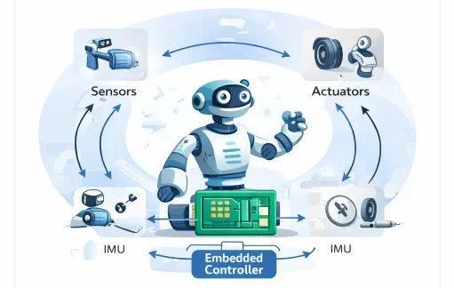
This architecture demonstrates the strict closed-loop timing governing robotic systems. Environmental sensors (e.g., optical encoders, IMUs, torque load cells) acquire physical states and stream data into an embedded microcontroller via deterministic buses. The processor executes discrete digital control algorithms within hard deadlines, transmitting drive signals via PWM or fieldbuses to physical actuators. Any unmodeled delay, task preemption jitter, or bus transmission latency degrades phase margin, destabilizing the physical plant.
Interactive Quick Review: Real-Time Systems & Control Timing
Test your understanding of hard versus soft real-time requirements and control loop execution before exploring discrete-time math:
1. What is the fundamental difference between hard real-time and soft real-time requirements in embedded robotics?
Answer: In hard real-time systems, missing a single deadline results in total system failure or catastrophic physical damage (such as a balancing inverted pendulum falling or an aerial vehicle crashing). In soft real-time systems, missing deadlines degrades quality of service or performance without causing complete failure.
2. Why can computation delays (\(\Delta t\)) destabilize a feedback control system even if the underlying control equations are mathematically optimal?
Answer: Delay introduces an unmodeled transport phase lag (\(\phi_{\text{lag}} = \omega \Delta t\)) into the open-loop transfer function, which erodes the phase margin and triggers destructive high-frequency limit-cycle oscillations.
Glossary of Key Terminology
Essential technical foundations governing embedded processors, RTOS kernels, and deterministic robotic communication networks:
Control Loop Timing and Transport Delay
Most robotic actuators are driven by discrete digital controllers executing periodic feedback routines. At each discrete interval \(k \in \mathbb{Z}^+\), the error vector \(\mathbf{e}[k]\) is mapped to control command \(\mathbf{u}[k]\):
$$\mathbf{u}[k] = K_p \mathbf{e}[k] + K_d \frac{\mathbf{e}[k] - \mathbf{e}[k-1]}{T_s} + K_i \sum_{j=0}^{k} \mathbf{e}[j] T_s$$If sensor acquisition, bus transmission, or processor computation introduces an uncompensated delay \(\tau_d\), the continuous-time feedback path incorporates a dead-time transport lag \(e^{-s \tau_d}\). In the frequency domain, this dead time alters open-loop transfer function \(L(s)\):
$$L_{\text{delayed}}(s) = L(s) e^{-s \tau_d} \quad \Rightarrow \quad \angle L_{\text{delayed}}(j\omega) = \angle L(j\omega) - \omega \tau_d$$The resulting phase margin erosion (\(\Delta \Phi = \omega_c \tau_d\), where \(\omega_c\) is the gain crossover frequency) shifts closed-loop system poles toward the right-half \(s\)-plane (\(s = \sigma + j\omega\)), inducing instability.
State-Space Discretization and Numerical Stability
Physical plant dynamics expressed in continuous-time state-space form:
$$\dot{\mathbf{x}}(t) = \mathbf{A}\mathbf{x}(t) + \mathbf{B}\mathbf{u}(t), \quad \mathbf{y}(t) = \mathbf{C}\mathbf{x}(t) + \mathbf{D}\mathbf{u}(t)$$are mapped into discrete-time state-space representations for digital embedded execution under a Zero-Order Hold (ZOH) assumption over sampling period \(T_s\):
$$\mathbf{x}[k+1] = \mathbf{A}_d \mathbf{x}[k] + \mathbf{B}_d \mathbf{u}[k]$$The discrete system matrices are calculated using the matrix exponential:
$$\mathbf{A}_d = e^{\mathbf{A} T_s} = \mathbf{I} + \mathbf{A}T_s + \frac{\mathbf{A}^2 T_s^2}{2!} + \dots = \sum_{k=0}^{\infty} \frac{(\mathbf{A}T_s)^k}{k!}$$ $$\mathbf{B}_d = \int_0^{T_s} e^{\mathbf{A}\eta} d\eta \, \mathbf{B} = \mathbf{A}^{-1}(e^{\mathbf{A} T_s} - \mathbf{I})\mathbf{B}$$A continuous linear system is asymptotically stable if all eigenvalues \(\lambda_i(\mathbf{A})\) satisfy \(\text{Re}(\lambda_i) < 0\). For the discrete equivalent, asymptotic stability requires that all discrete eigenvalues \(\mu_i(\mathbf{A}_d)\) lie strictly inside the complex unit circle:
$$|\mu_i| = \left|e^{\lambda_i T_s}\right| < 1 \quad \forall i$$To preserve phase margin and avoid high-frequency aliasing, the sampling rate \(f_s = 1/T_s\) must satisfy the empirical guideline \(f_s \ge 10 f_b\) to \(30 f_b\), where \(f_b\) is the closed-loop system bandwidth.
Real-Time Task Scheduling Algorithms
Robotic microcontrollers run concurrent tasks (motor current loops, trajectory interpolation, kinematics, safety monitoring, telemetry). Schedulability analysis guarantees that every task meets its operational deadline.
Rate Monotonic Scheduling (RMS)
RMS assigns static priorities inversely proportional to task periods (\(T_1 < T_2 \Rightarrow \text{Priority}_1 > \text{Priority}_2\)). For \(n\) independent periodic tasks with worst-case execution times \(C_i\) and periods \(T_i\), the Liu and Layland utilization bound guarantees schedulability if:
$$U = \sum_{i=1}^{n} \frac{C_i}{T_i} \le n \left( 2^{1/n} - 1 \right)$$As \(n \to \infty\), the bound converges asymptotically:
$$\lim_{n \to \infty} n \left( 2^{1/n} - 1 \right) = \ln(2) \approx 0.6931 \quad (69.31\%)$$Earliest Deadline First (EDF)
EDF assigns priorities dynamically: whichever task has the nearest absolute deadline is assigned highest execution priority. For independent periodic tasks with deadlines equal to periods (\(D_i = T_i\)), EDF achieves full processor utilization:
$$\sum_{i=1}^{n} \frac{C_i}{T_i} \le 1.0 \quad (100\%)$$Engineering Challenges & Technical Solutions
Deploying deterministic real-time control software on embedded physical hardware involves resolving several critical timing, hardware, and concurrency challenges:
The Challenge: When a low-priority task acquires a shared mutex (e.g., an SPI bus interface) and is preempted by a medium-priority background thread, a critical high-priority control loop requiring that mutex is blocked indefinitely, causing hard deadline misses.
- Priority Inheritance Protocol (PIP): The low-priority mutex owner temporarily inherits the priority of the highest-priority thread waiting on the resource until it unlocks the mutex.
- Priority Ceiling Protocol (PCP): Each semaphore is assigned a priority ceiling equal to the highest priority task that may lock it, preventing chained blocking and eliminating deadlocks offline.
The Challenge: Standard Linux kernels utilize virtual memory paging, coarse timers, and non-preemptible spinlocks that induce multi-millisecond scheduling jitter, making them unsuitable for 1 kHz motor commutation.
- PREEMPT_RT Kernel Patch: Converts in-kernel spinlocks into sleeping preemptible mutexes, enforces threaded interrupt handlers, and provides microsecond-bounded latency.
- Asymmetric Multiprocessing (AMP) / Co-Processor Architectures: High-level navigation and perception run on Linux/ROS on ARM Cortex-A application cores, while deterministic motor control loops run bare-metal or on FreeRTOS on dedicated Cortex-M or FPGA cores.
The Challenge: CAN bus networks use non-destructive bitwise arbitration (CSMA/CA). During periods of heavy bus load, lower-priority actuator message frames experience transmission delays, leading to missing or jittered motor torque setpoints.
- EtherCAT Processing on the Fly: Master frames circulate through slave nodes, which read inputs and write output data within nanoseconds at the hardware level, keeping cycle times under \(100\ \mu\text{s}\).
- Time-Triggered Communication (TTCAN / TSN): Allocates static, globally synchronized TDMA time slots to eliminate message collisions and transmission jitter entirely.
The Challenge: High-frequency sensor streams (e.g., quadrature encoders, high-speed ADCs) triggering interrupts at 100 kHz can overwhelm the CPU with context-switching overhead, starving the main control thread.
- Direct Memory Access (DMA): Hardware DMA controllers stream incoming ADC or SPI data directly into circular RAM buffers without CPU intervention, generating an interrupt only upon buffer completion.
- Hardware Quadrature Encoders: Dedicated on-chip timer modules decode quadrature pulses in silicon hardware, eliminating software ISR execution for position tracking.
Interactive Quick Review: Scheduling, Discretization & Networks
Reinforce key concepts regarding Rate Monotonic bounds, zero-order hold discretization, and bus communication latency before reviewing the FAQ:
1. What is the maximum utilization bound for Rate Monotonic Scheduling (RMS) as task count \(n\) approaches infinity?
Answer: As \(n \to \infty\), the Liu and Layland RMS utilization bound approaches \(\ln(2) \approx 0.693\) (69.3%), guaranteeing schedulability for any independent periodic task set whose total utilization is below this threshold.
2. Why must communication latency (\(\tau_c\)) on industrial fieldbuses remain strictly smaller than sampling time (\(T_s\))?
Answer: If communication latency exceeds \(T_s\), the controller operates on stale sensor data. This introduces variable time jitter, reduces feedback phase margin, and can cause instability in closed-loop systems.
External References and Further Reading
To explore real-time operating systems, embedded hardware architectures, and deterministic scheduling theory, consult these authoritative resources:
- FreeRTOS Official Documentation – Industry-standard open-source Real-Time Operating System for microcontrollers, featuring micro-kernel architecture and task scheduling guides.
- EtherCAT Technology Group (ETG) – Technical specifications for deterministic Ethernet-based fieldbus communication used in industrial robotics.
- ARM Cortex-M Embedded Processor Architecture – Hardware reference manuals detailing NVIC interrupt latency, hardware FPUs, and real-time execution pipelines.
Frequently Asked Questions about Real-Time Embedded Systems in Robotics
What is the difference between a microcontroller (MCU) and a single-board computer (SBC) in robotics?
Microcontrollers (e.g., ARM Cortex-M, STM32) execute bare-metal firmware or RTOS tasks with deterministic microsecond-level timing for low-level motor PWM, encoder reading, and PID loops. Single-Board Computers (e.g., NVIDIA Jetson, Raspberry Pi) run full operating systems (Linux/ROS) to handle high-level computer vision, SLAM, and path planning tasks.
Why is a standard desktop Linux kernel unsuitable for hard real-time robot control?
Standard Linux OS kernels prioritize throughput and user fairness over determinism. Virtual memory page faults, thread context switching, and non-preemptible kernel drivers introduce millisecond-scale timing jitter that can destabilize high-frequency feedback loops.
How does PREEMPT_RT transform standard Linux into a real-time OS?
The PREEMPT_RT patch converts Linux kernel spinlocks and interrupt handlers into preemptible mutexes. This allows high-priority real-time threads to preempt lower-priority kernel activities immediately, providing bounded microsecond-level scheduling determinism.
What is priority inversion, and how do RTOS kernels prevent it?
Priority inversion occurs when a low-priority task holds a shared resource mutex needed by a high-priority task, while a medium-priority task preempts the low-priority task, indirectly starving the high-priority task. RTOS kernels resolve this using Priority Inheritance Protocols, temporarily elevating the low-priority task's priority to match the blocked high-priority task until the mutex is released.
End-of-Page Exercises: Review, Thought-Provoking & Engineering Problems
Section 1: Foundational Review Questions & Answers
1. What defines a hard real-time system in embedded control?
Answer: A system where missing a single timing deadline causes complete operational failure or physical damage.
2. What is the mathematical discrete-time control equation for proportional error feedback?
Answer: \(u[k] = K e[k]\), mapping discrete tracking error at step \(k\) directly to control output.
3. How is a continuous state matrix \(\mathbf{A}\) converted to a discrete-time matrix \(\mathbf{A}_d\) for a sampling interval \(T_s\)?
Answer: Via the matrix exponential function: \(\mathbf{A}_d = e^{\mathbf{A} T_s}\).
4. What standard rule-of-thumb relates sampling frequency (\(f_s\)) to dominant system bandwidth (\(f_b\))?
Answer: Sampling frequency should be at least ten times the dominant system bandwidth: \(f_s \ge 10 f_b\).
5. What formula determines processor utilization \(U\) for \(n\) periodic real-time tasks?
Answer: \(U = \sum_{i=1}^{n} (C_i / T_i)\), summing the execution-time-to-period ratios across all tasks.
6. What condition must interrupt latency (\(T_{\text{latency}}\)) satisfy for reliable sensor data capture?
Answer: Interrupt response latency must be less than or equal to the maximum allowable deadline: \(T_{\text{latency}} \le T_{\text{deadline}}\).
7. What requirement governs communication network delay (\(\tau_c\)) relative to control sampling time (\(T_s\))?
Answer: Communication network transmission delay must remain strictly less than the sampling period: \(\tau_c < T_s\).
8. Name three industrial deterministic communication networks widely utilized in robotics.
Answer: Controller Area Network (CAN), EtherCAT, and Time-Sensitive Networking (TSN).
9. What hardware architecture is commonly selected for parallel, zero-jitter execution?
Answer: Field Programmable Gate Arrays (FPGAs).
10. Name two primary real-time task scheduling algorithms utilized in embedded RTOS micro-kernels.
Answer: Rate Monotonic Scheduling (RMS) and Earliest Deadline First (EDF).
Section 2: Analytical & Thought-Provoking Questions
1. Why can a high-performance desktop processor running Linux fail at 1 kHz motor control while a modest 160 MHz ARM Cortex-M microcontroller succeeds?
Answer: Embedded motor control demands temporal determinism rather than raw floating-point throughput. Desktop processors running general-purpose operating systems experience non-deterministic cache misses, power-saving frequency throttling, and OS kernel thread preemptions that introduce random millisecond-level scheduling jitter, whereas microcontrollers feature hardware interrupt controllers (NVIC) and deterministic execution pipelines that respond in exact clock cycles.
2. How does execution timing jitter introduce unmodeled noise and instability into digital derivative control?
Answer: Digital derivative control approximates velocity as \(v[k] = (e[k] - e[k-1]) / T_s\) assuming constant step duration \(T_s\). When execution timing jitters, dividing by a constant \(T_s\) when actual elapsed time varied creates artificial numerical velocity spikes, injecting high-frequency noise into actuator torque outputs and causing motor buzzing or physical resonance.
3. What mechanical risks occur when an embedded microcontroller suffers an unhandled memory corruption or stack overflow error?
Answer: Stack overflow overwrites function return addresses and control variables in RAM. Without fail-safe hardware memory protection (MPU) or watchdog reset interlocks, corrupt memory can freeze PWM gate signals at 100% duty cycle, driving motor actuators at full power into physical mechanical hard stops or human operators.
4. Why is Rate Monotonic Scheduling (RMS) classified as static while Earliest Deadline First (EDF) is dynamic?
Answer: RMS assigns task priorities offline based strictly on periodic rates (shorter period = higher fixed priority). EDF evaluates deadlines dynamically at runtime during every scheduling decision, assigning highest priority to whichever active task's absolute deadline is nearest in time, enabling EDF to reach 100% processor utilization.
5. How do zero-order hold (ZOH) DAC converters introduce an inherent half-sample time delay into feedback loops?
Answer: A ZOH holds a constant discrete control voltage flat over the entire sampling interval \([k T_s, (k+1) T_s]\). Averaging this step output over time reveals that the continuous signal equivalent lags the instantaneous mathematical control target by exactly half the sampling interval (\(T_s/2\)), eroding phase margin in fast physical control systems.
6. Why is nested interrupt vector controller (NVIC) hardware design critical for sub-microsecond sensor response?
Answer: Hardware NVIC controllers automatically handle interrupt preemption, priority decoding, and register state saving (tail-chaining) directly in silicon hardware without software overhead, allowing emergency safety signals (e.g., optical encoder limit trips) to preempt active motor loops within 12 clock cycles.
7. How does time-triggered architecture (TTA) eliminate message arbitration collision contention on CAN networks?
Answer: Standard CAN uses priority-based CSMA/CA arbitration where high-priority messages delay lower-priority frames non-deterministically. Time-triggered communication enforces a strict globally synchronized TDMA time-slot schedule, assigning dedicated millisecond transmission windows to each node and eliminating bus contention entirely.
8. Why is hardware-in-the-loop (HIL) testing mandatory for safety-critical embedded robotics software?
Answer: Pure software simulation ignores hardware microsecond clock drift, bus latency, and silicon pin electrical characteristics. HIL connects actual physical embedded microcontroller hardware to real-time FPGA physics simulators, verifying firmware timing, interrupt handling, and fault recovery before physical deployment.
9. What causes tick-loss drift in RTOS timekeeping, and how do 64-bit hardware timers prevent it?
Answer: Software RTOS timekeeping relies on periodic timer interrupt "ticks" (e.g., 1 ms). If long critical sections disable global interrupts, timer ticks are missed, causing internal system time to drift behind real physical time. Hardware 64-bit free-running timers count continuously in silicon regardless of CPU interrupt status, eliminating time drift.
10. How does memory management unit (MMU) virtual paging degrade real-time determinism?
Answer: MMUs map virtual memory addresses to physical RAM pages. When a real-time thread accesses a page swapped to disk or unallocated, the CPU triggers a Translation Lookaside Buffer (TLB) miss page fault interrupt, stalling process execution for milliseconds while the OS kernel loads memory pages. Real-time threads must lock physical RAM (using mlockall()) to eliminate page faults.
11. Why do autonomous mobile robots combine bare-metal microcontrollers with ROS 2 micro-agents (micro-ROS)?
Answer: Bare-metal microcontrollers excel at low-latency motor control and hardware sensor reading, but lack rich middleware networking protocols. Micro-ROS lightweight client libraries allow low-power microcontrollers to publish sensor topics and receive motor commands directly on ROS 2 DDS networks while retaining deterministic RTOS scheduling loops.
12. How does asymmetry between worst-case (WCET) and best-case (BCET) execution paths complicate scheduling design?
Answer: Complex control code with conditional branching or iterative matrix solvers can execute rapidly under normal states (BCET) but require extensive iterations during edge cases (WCET). Schedulability proofs must provision system capacity conservatively for WCET to guarantee hard deadlines, leaving significant processor capacity idle during typical operations.
Section 3: Numerical Engineering Problems & Solutions
A continuous-time 1-DOF joint velocity system is modeled as \(\dot{x}(t) = -5.0 x(t)\). The system is implemented digitally on an ARM Cortex microcontroller operating at a sampling period \(T_s = 0.04\text{ seconds}\). Calculate the discrete system transition constant \(A_d = e^{A T_s}\), write the discrete state equation \(x[k+1] = A_d x[k]\), and compute the state value \(x[1]\) if the initial state is \(x[0] = 10.0\text{ rad/s}\).
1. Calculate the exponent: $$A T_s = -5.0 \times 0.04 = -0.20$$ 2. Compute the scalar exponential: $$A_d = e^{-0.20} \approx 0.81873$$ 3. Formulate discrete state equation: $$x[k+1] = 0.81873 \, x[k]$$ 4. Compute state \(x[1]\): $$x[1] = 0.81873 \times 10.0\text{ rad/s} = 8.1873\text{ rad/s}$$ Final Answer: Discrete matrix constant is \(A_d \approx 0.8187\) and state \(x[1]\) is \(8.19\text{ rad/s}\).
An embedded quadrotor flight controller executes three periodic tasks under Rate Monotonic Scheduling (RMS):
- Task 1 (IMU & Motor Loop): \(C_1 = 0.2\text{ ms}\), \(T_1 = 1.0\text{ ms}\)
- Task 2 (Attitude Estimator): \(C_2 = 0.5\text{ ms}\), \(T_2 = 2.5\text{ ms}\)
- Task 3 (Telemetry Output): \(C_3 = 1.0\text{ ms}\), \(T_3 = 10.0\text{ ms}\)
1. Calculate task utilization ratios: $$U_1 = \frac{0.2}{1.0} = 0.20, \quad U_2 = \frac{0.5}{2.5} = 0.20, \quad U_3 = \frac{1.0}{10.0} = 0.10$$ 2. Sum total processor utilization: $$U = 0.20 + 0.20 + 0.10 = 0.50 \quad (50\%)$$ 3. Compute Liu & Layland RMS bound for \(n = 3\): $$U_{\text{bound}} = 3\left(2^{1/3} - 1\right) = 3(1.25992 - 1) = 3(0.25992) \approx 0.7798 \quad (77.98\%)$$ 4. Compare utilization against theoretical threshold: $$0.50 \le 0.7798 \Rightarrow \text{Schedulability is guaranteed}$$ Final Answer: Total utilization is \(0.50\ (50\%)\); because \(0.50 \le 0.7798\), the task set is guaranteed schedulable under RMS.
A high-speed industrial robotic manipulator joint has a dominant physical closed-loop system bandwidth of \(f_b = 45\text{ Hz}\). Apply the engineering sampling guideline \(f_s \ge 10 f_b\) to calculate the minimum required sampling frequency \(f_s\) in Hz and determine the corresponding maximum allowable discrete sampling period \(T_s\) in milliseconds.
1. Minimum sampling frequency: $$f_s = 10 \times f_b = 10 \times 45\text{ Hz} = 450\text{ Hz}$$ 2. Maximum allowable sampling interval: $$T_s = \frac{1}{f_s} = \frac{1}{450}\text{ s} \approx 0.002222\text{ seconds}$$ 3. Convert interval to milliseconds: $$T_s = 0.002222\text{ s} \times 1000\text{ ms/s} \approx 2.22\text{ ms}$$ Final Answer: Minimum sampling frequency is \(450\text{ Hz}\), requiring a maximum sampling interval of \(2.22\text{ ms}\).
An EtherCAT fieldbus connects an embedded central controller to joint servo drives operating at a control loop sampling interval of \(T_s = 250\ \mu\text{s}\). Hardware benchmarks indicate frame propagation delay is \(\tau_{\text{prop}} = 45\ \mu\text{s}\), processing time is \(\tau_{\text{proc}} = 85\ \mu\text{s}\), and packet jitter is \(\tau_{\text{jitter}} = 30\ \mu\text{s}\). Calculate total communication latency \(\tau_c = \tau_{\text{prop}} + \tau_{\text{proc}} + \tau_{\text{jitter}}\), verify if \(\tau_c < T_s\) holds, and determine the remaining timing margin.
1. Calculate total network latency: $$\tau_c = 45\ \mu\text{s} + 85\ \mu\text{s} + 30\ \mu\text{s} = 160\ \mu\text{s}$$ 2. Verify stability boundary: $$160\ \mu\text{s} < 250\ \mu\text{s} \Rightarrow \text{Condition holds}$$ 3. Calculate remaining timing headroom: $$\text{Margin} = T_s - \tau_c = 250\ \mu\text{s} - 160\ \mu\text{s} = 90\ \mu\text{s}$$ Final Answer: Total communication latency is \(160\ \mu\text{s}\), preserving closed-loop stability with a \(90\ \mu\text{s}\) timing margin.
A magnetic joint encoder generates a hardware interrupt service request (ISR) upon index marker detection. Processor hardware register stacking requires \(T_{\text{stack}} = 1.2\ \mu\text{s}\), and the ISR execution routine takes \(T_{\text{exec}} = 3.5\ \mu\text{s}\). If the encoder timing deadline requires data processing within \(T_{\text{deadline}} = 8.0\ \mu\text{s}\) to prevent pulse miscounting, calculate total interrupt latency \(T_{\text{latency}}\) and the remaining deadline margin.
1. Calculate total interrupt response latency: $$T_{\text{latency}} = T_{\text{stack}} + T_{\text{exec}} = 1.2\ \mu\text{s} + 3.5\ \mu\text{s} = 4.7\ \mu\text{s}$$ 2. Verify against deadline limit: $$4.7\ \mu\text{s} \le 8.0\ \mu\text{s} \Rightarrow \text{Requirement satisfied}$$ 3. Compute remaining safety headroom: $$\text{Margin} = T_{\text{deadline}} - T_{\text{latency}} = 8.0\ \mu\text{s} - 4.7\ \mu\text{s} = 3.3\ \mu\text{s}$$ Final Answer: Total interrupt latency is \(4.7\ \mu\text{s}\), leaving a \(3.3\ \mu\text{s}\) deadline margin.
A \(200\text{ Hz}\) sinusoidal motor current control loop experiences an embedded execution transport delay of \(\Delta t = 0.5\text{ milliseconds}\) (\(0.0005\text{ s}\)). Calculate the uncompensated feedback phase lag angle \(\phi_{\text{lag}} = \omega \Delta t\) in radians and degrees.
1. Angular frequency: $$\omega = 2 \pi f = 2 \times \pi \times 200\text{ Hz} \approx 1256.64\text{ rad/s}$$ 2. Calculate phase lag in radians: $$\phi_{\text{lag}} = \omega \Delta t = 1256.64\text{ rad/s} \times 0.0005\text{ s} \approx 0.6283\text{ radians}$$ 3. Convert radians to degrees: $$\phi_{\text{deg}} = 0.6283\text{ rad} \times \frac{180^\circ}{\pi} \approx 36.0^\circ$$ Final Answer: Transport delay introduces an uncompensated phase lag of \(0.628\text{ rad}\ (36.0^\circ)\).
A discrete-time joint position controller has a discrete state transition matrix \(\mathbf{A}_d\) with complex conjugate eigenvalues \(\mu_{1,2} = 0.60 \pm 0.70 j\). Calculate the eigenvalue magnitude \(|\mu| = \sqrt{\text{Re}^2 + \text{Im}^2}\) and state whether the discrete closed-loop system is asymptotically stable.
1. Extract real and imaginary components: $$\text{Re} = 0.60, \quad \text{Im} = 0.70$$ 2. Compute modulus: $$|\mu| = \sqrt{(0.60)^2 + (0.70)^2} = \sqrt{0.36 + 0.49} = \sqrt{0.85} \approx 0.9220$$ 3. Apply unit circle stability criterion: $$|\mu| \approx 0.922 < 1.0 \Rightarrow \text{System is stable}$$ Final Answer: Eigenvalue modulus is \(|\mu| \approx 0.922\); because \(|\mu| < 1.0\), the discrete system is asymptotically stable.
An industrial CAN bus operating at a transmission baud rate of \(B = 500,000\text{ bits/second}\) (500 kbps) transmits an 11-bit identifier frame containing an 8-byte payload. Including bit stuffing, the total message length is \(L_{\text{frame}} = 125\text{ bits}\). Calculate the transmission time \(T_{\text{frame}}\) of the message across the physical bus in microseconds.
1. Transmission time formula: $$T_{\text{frame}} = \frac{L_{\text{frame}}}{B}$$ 2. Substitute numerical values: $$T_{\text{frame}} = \frac{125\text{ bits}}{500,000\text{ bits/s}} = 0.000250\text{ seconds}$$ 3. Convert seconds to microseconds: $$T_{\text{frame}} = 0.000250\text{ s} \times 10^6\ \mu\text{s/s} = 250\ \mu\text{s}$$ Final Answer: CAN frame transmission duration is \(250\ \mu\text{s}\).
An independent hardware Watchdog Timer (WDT) is clocked by an internal \(32\text{ kHz}\) (\(32,000\text{ Hz}\)) oscillator. Safety regulations require the WDT to trigger a hardware reset if firmware fails to refresh the counter within \(T_{\text{timeout}} = 50\text{ milliseconds}\) (\(0.050\text{ s}\)). Calculate the reload count value \(N_{\text{count}} = f_{\text{clock}} \times T_{\text{timeout}}\).
1. Identify clock frequency: $$f_{\text{clock}} = 32,000\text{ ticks/s}$$ 2. Calculate tick reload threshold: $$N_{\text{count}} = 32,000 \times 0.050 = 1,600\text{ ticks}$$ Final Answer: The hardware WDT reload threshold must be configured to \(1,600\text{ ticks}\).
A 12-bit ADC samples an analog motor current sensing voltage changing at a maximum slew rate of \(dV/dt = 500\text{ V/s}\). Microcontroller clock jitter introduces a sampling aperture uncertainty of \(\Delta t_{\text{jitter}} = 2.0\text{ nanoseconds}\) (\(2.0 \times 10^{-9}\text{ s}\)). Calculate the peak amplitude voltage error \(\Delta V = (dV/dt) \times \Delta t_{\text{jitter}}\) in microvolts (\(\mu\text{V}\)).
1. Voltage error formulation: $$\Delta V = 500\text{ V/s} \times (2.0 \times 10^{-9}\text{ s}) = 1.0 \times 10^{-6}\text{ Volts}$$ 2. Convert to microvolts: $$\Delta V = 1.0 \times 10^{-6}\text{ V} \times 10^6\ \mu\text{V/V} = 1.0\ \mu\text{V}$$ Final Answer: Aperture jitter induces an amplitude error of \(1.0\ \mu\text{V}\).
An engineer adds a fourth periodic task (\(C_4 = 2.0\text{ ms}\), \(T_4 = 8.0\text{ ms}\)) to an existing real-time system with current total utilization \(U_{\text{prev}} = 0.55\). Calculate the new task utilization \(U_4\), determine the updated total utilization \(U_{\text{new}}\), and check whether the processor is overloaded (\(U > 1.0\)).
1. Calculate additional task utilization: $$U_4 = \frac{C_4}{T_4} = \frac{2.0\text{ ms}}{8.0\text{ ms}} = 0.25 \quad (25\%)$$ 2. Sum total utilization: $$U_{\text{new}} = U_{\text{prev}} + U_4 = 0.55 + 0.25 = 0.80 \quad (80\%)$$ 3. Overload evaluation: $$0.80 \le 1.0 \Rightarrow \text{Processor capacity is sufficient}$$ Final Answer: Updated total utilization is \(0.80\ (80\%)\); the task set remains CPU-feasible.
A robotic microcontroller reads 1,000 sensor bytes per control cycle. Under CPU-driven interrupt polling, handling each byte consumes 15 clock cycles. Using hardware Direct Memory Access (DMA), transfer setup requires a flat 50 clock cycles for the entire 1,000-byte block. Calculate the total CPU cycles under polling, cycles under DMA, and the percentage reduction in CPU cycle consumption.
1. CPU cycles consumed under polling: $$N_{\text{poll}} = 1000\text{ bytes} \times 15\text{ cycles/byte} = 15,000\text{ cycles}$$ 2. CPU cycles consumed under DMA: $$N_{\text{DMA}} = 50\text{ cycles}$$ 3. Percentage reduction: $$\% \text{ Savings} = \frac{15,000 - 50}{15,000} \times 100 = \frac{14,950}{15,000} \times 100 \approx 99.67\%$$ Final Answer: DMA reduces processor overhead from 15,000 to 50 cycles, achieving a \(99.67\%\) reduction in CPU cycle consumption.
Real-Time Embedded Systems in Robotics — Summary & Wrap-Up
Real-time embedded systems provide the deterministic computational foundation that enables physical robots to operate safely and predictably. By enforcing hard deadline bounds, discrete state discretization, Rate Monotonic and EDF task scheduling, low-latency interrupt handling, and deterministic fieldbus communications (CAN, EtherCAT), embedded systems engineers guarantee that complex control theory operates with microsecond precision in real-world physical machines.
Explore Robotics Software and Infrastructure
Real-time embedded systems operate within a broader robotics software architecture that includes simulation platforms, middleware communication frameworks, distributed computing environments, and cloud-connected learning systems. Together, these technologies enable robots to move from virtual experimentation to reliable physical deployment.
Robot Operating System (ROS and ROS 2)
ROS provides the communication framework that connects embedded controllers with perception, planning, and coordination modules.
Robotics Simulation Platforms
Simulation environments allow algorithms and control strategies to be tested safely before deployment on real hardware.
Robotics Middleware and Distributed Systems
Middleware systems coordinate communication among distributed robotic subsystems and computational modules.
Robotic Digital Twin Systems and Simulation
Digital twin models synchronize simulated robots with physical machines to monitor performance and evaluate design changes.
Cloud Robotics and Edge Intelligence
Cloud and edge computing architectures extend robotic capabilities through shared data processing and distributed intelligence.