
Before an autonomous machine moves in the physical world, it almost always moves in virtual simulation first. Robotics simulation platforms provide the software infrastructure required to model kinematics, multi-body physical dynamics, environmental contact constraints, and perception sensors without risking catastrophic damage to expensive hardware prototypes.
Simulation functions as the digital proving ground for modern autonomous robotics. Within high-fidelity virtual worlds, engineers evaluate trajectory planners, tune feedback control gains, stress-test fault-recovery logic, and train deep reinforcement learning policies across billions of interaction steps long before hardware fabrication and physical field deployment.
In reinforcement learning workflows, parallelized physics simulation enables training regimes that would take decades of physical wall-clock time to be compressed into hours of GPU compute. By eliminating hardware wear and collision hazards, simulation platforms accelerate innovation cycles and lower research barriers.
However, virtual simulation represents only one layer of a complete robotics software architecture. Virtual models must bridge seamlessly to middleware transport layers, deterministic real-time embedded controllers, Hardware-in-the-Loop testbeds, and cloud fleet learning backends before virtual algorithms can operate reliably on physical robots.
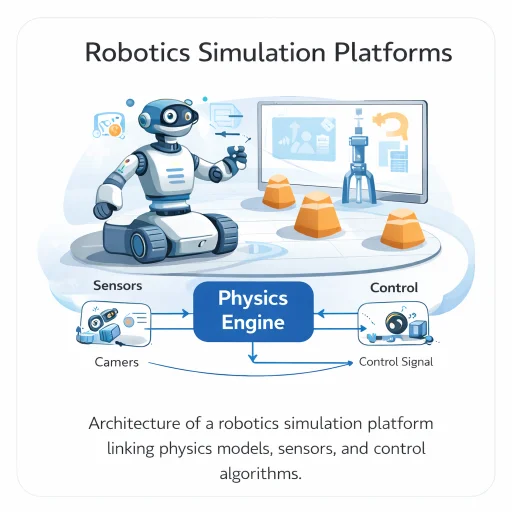
This architecture illustrates the computational dataflow governing modern robotics simulation platforms. A digital model of the robot interacts with a numerical multi-body physics engine that resolves equations of motion, gravitational vectors, and joint constraint reactions. Sensor emulation pipelines generate synthetic camera frames, LiDAR point clouds, and IMU telemetry with additive noise profiles. These synthetic signals feed perception and control algorithms, which return joint torque setpoints to the simulated plant, closing the virtual feedback loop.
Interactive Quick Review: Simulation Fundamentals
Test your understanding of virtual prototyping and physics engine integration before exploring numerical integration mathematics:
1. What is the primary operational purpose of a robotics simulation platform?
Answer: Simulation platforms provide virtual experimental environments to test kinematics, control laws, perception algorithms, and reinforcement learning policies repeatedly and at high speed without physical hardware damage.
2. Why are physics engines required inside robotics simulation platforms?
Answer: Physics engines numerically integrate Newton-Euler and Lagrangian dynamic equations to approximate physical motion, gravity, inertia, friction, and contact forces acting on virtual rigid bodies.
Glossary of Key Terminology
Essential mathematical, computational, and mechanical definitions governing robotics simulation platforms, physics engines, and sim-to-real transfer:
Physics Engines & Numerical Multi-Body Dynamics
At the core of every modern robotics simulation platform lies a numerical physics solver. The physics engine computes joint accelerations and body trajectories by solving the non-linear multi-body equations of motion:
$$\mathbf{M}(\mathbf{q})\ddot{\mathbf{q}} + \mathbf{C}(\mathbf{q}, \dot{\mathbf{q}})\dot{\mathbf{q}} + \mathbf{G}(\mathbf{q}) + \mathbf{J}_c^T(\mathbf{q})\boldsymbol{\lambda}_c = \boldsymbol{\tau}$$where \(\mathbf{q} \in \mathbb{R}^n\) represents the generalized joint coordinate vector, \(\mathbf{M}(\mathbf{q})\) is the symmetric positive-definite mass matrix, \(\mathbf{C}(\mathbf{q}, \dot{\mathbf{q}})\) is the Coriolis and centrifugal matrix, \(\mathbf{G}(\mathbf{q})\) is the gravitational torque vector, \(\boldsymbol{\tau}\) is the actuator command vector, and \(\mathbf{J}_c^T \boldsymbol{\lambda}_c\) maps external contact constraint forces \(\boldsymbol{\lambda}_c\) into joint torques via the contact Jacobian \(\mathbf{J}_c\).
Because closed-form analytical solutions to coupled multi-body systems do not exist, the physics engine isolates accelerations and advances time discretely using numerical integration schemes:
$$\ddot{\mathbf{q}} = \mathbf{M}^{-1}(\mathbf{q}) \left[ \boldsymbol{\tau} - \mathbf{C}(\mathbf{q}, \dot{\mathbf{q}})\dot{\mathbf{q}} - \mathbf{G}(\mathbf{q}) - \mathbf{J}_c^T \boldsymbol{\lambda}_c \right]$$Explicit vs. Semi-Implicit Numerical Integration
Standard explicit Euler integration updates states sequentially using values evaluated at the current time step \(k\):
$$\mathbf{q}_{k+1} = \mathbf{q}_k + \dot{\mathbf{q}}_k \Delta t, \quad \dot{\mathbf{q}}_{k+1} = \dot{\mathbf{q}}_k + \ddot{\mathbf{q}}_k \Delta t$$Explicit Euler is computationally fast per step but introduces numerical energy growth, making it conditionally stable. Robotics simulators favor semi-implicit Euler (symplectic Euler), which evaluates velocity updates first and uses the advanced velocity to integrate positions:
$$\dot{\mathbf{q}}_{k+1} = \dot{\mathbf{q}}_k + \ddot{\mathbf{q}}_k \Delta t, \quad \mathbf{q}_{k+1} = \mathbf{q}_k + \dot{\mathbf{q}}_{k+1} \Delta t$$This formulation preserves phase-space volume and guarantees structural energy conservation for unforced Hamiltonian systems.
Numerical Stability Criteria & Contact Mechanics
In virtual simulations, numerical integration stability is bounded by the highest natural oscillation frequency \(\omega_{\max}\) present in the robotic system (e.g., stiff joint springs, high-gain PID feedback loops, or rigid contact boundaries):
$$\ddot{x}(t) + \omega^2 x(t) = 0$$For explicit integration schemes, the stability domain requires the discrete time step \(\Delta t\) to remain strictly bounded:
$$\Delta t < \frac{2}{\omega_{\max}}$$If \(\Delta t \ge 2/\omega_{\max}\), the numerical eigenvalues cross outside the unit circle in the complex plane, injecting artificial numerical energy that causes simulated joints and colliding meshes to violently diverge.
Contact & Collision Force Formulations
To model interaction dynamics during robotic grasping, foot-ground impacts, or tool contact, simulators employ regularized spring-damper models or constraint-based Linear Complementarity Problem (LCP) formulations. Under the Hunt-Crossley regularized contact model, normal contact force \(F_n\) is defined as:
$$F_n = k \delta^n + c(\delta) \dot{\delta}$$where \(\delta\) denotes surface penetration depth, \(k\) is the contact surface stiffness coefficient, and \(c(\delta)\) is the non-linear penetration-dependent damping coefficient that prevents non-physical negative pull-off forces upon separation.
Engineering Challenges & Technical Solutions
Constructing high-fidelity, real-time robotics simulation platforms presents significant physical, algorithmic, and numerical engineering hurdles:
The Challenge: High contact stiffness (\(k \gg 0\)) creates stiff ordinary differential equations with massive natural frequencies \(\omega = \sqrt{k/m}\). Explicit solvers require microsecond step sizes to prevent numerical instability, causing severe simulation slowdown or mesh explosion.
- Projected Gauss-Seidel LCP Solvers: Formulating contacts as impulse-velocity complementarity constraints rather than penalty spring forces, resolving multi-point contacts stably at standard 1 ms time steps.
- Soft Constraint Regularization: Introducing numerical compliance matrices (\(\boldsymbol{\Sigma}\)) into the constraint equation \(\left(\mathbf{J}_c \mathbf{M}^{-1} \mathbf{J}_c^T + \boldsymbol{\Sigma}\right) \boldsymbol{\lambda}_c = \mathbf{b}\), preventing solver divergence near kinematic singularities.
The Challenge: Control policies trained purely within static virtual simulations often fail catastrophically upon physical robot deployment due to unmodeled motor backlash, cable compliance, micro-friction variations, and actuator saturation (\(\boldsymbol{\theta}_{\text{real}} \neq \boldsymbol{\theta}_{\text{sim}}\)).
- Domain Randomization (DR): Randomizing inertial properties, link centers of mass, joint friction, and communication latencies uniformly across training episodes to learn policies that remain robust to parameter mismatch.
- Sim-to-Real System Identification: Executing automated experimental physical trajectories to log motor currents, updating simulator physics parameters via non-linear least squares optimization.
The Challenge: Simulating dozens of visual RGB cameras and high-density 3D LiDAR scanners across multi-robot fleets creates severe graphics rendering bottlenecks, dragging simulation speeds below real-time.
- GPU Ray-Tracing Hardware Acceleration: Utilizing dedicated RT cores (e.g., NVIDIA OptiX in Isaac Sim) to parallelize millions of laser range queries and visual photon paths concurrently.
- Convex Hull Collision Simplification: Decoupling high-resolution visual meshes from simplified convex bounding hulls for physics checks using the GJK algorithm, cutting contact checks by over 95%.
The Challenge: In Hardware-in-the-Loop (HIL) architectures, packet serialization and network delay between the physical microcontroller and the simulation host erode phase margins in high-speed control loops.
- Deterministic Middleware & TSN: Deploying low-latency industrial transport buses (CAN FD, EtherCAT) and ROS 2 DDS middleware with Best-Effort QoS profiles, as described in Robot Operating System (ROS and ROS 2).
- Real-Time OS Kernel Pinning: Executing physics co-simulation engines on PREEMPT_RT Linux kernels with dedicated core pinning and memory locking (
mlockall), detailed in Real-Time Embedded Systems in Robotics.
Comparative Overview of Modern Simulation Engines
Modern robotics simulation platforms balance fidelity, rendering realism, scripting flexibility, and distributed scalability based on targeted application domains:
| Platform | Physics Backends | Primary Strengths | Target Applications |
|---|---|---|---|
| Gazebo (Ignition / Harmonic) | DART, Bullet, ODE, Tidy | Native ROS/ROS 2 integration, distributed node plugins, open-source ecosystem. | Academic research, mobile manipulation, outdoor field navigation. |
| NVIDIA Isaac Sim | PhysX 5 (GPU CUDA), Omniverse | RTX photorealistic ray-tracing, massive parallel RL envs (Isaac Lab), USD assets. | Deep reinforcement learning, synthetic data for vision, digital factory twins. |
| CoppeliaSim (V-REP) | MuJoCo, Bullet, ODE, Vortex | Kinematics solvers, multi-threaded cross-platform API, Lua/Python scripting. | Industrial workcells, manipulator path verification, educational curricula. |
| MuJoCo | Convex Contact Optimizer | Analytic contact derivatives, speed, minimal constraint violations. | Locomotion research, optimal trajectory control, biomechanics. |
Interactive Quick Review: Stability, Contact & Domain Randomization
Reinforce key concepts regarding Euler step limits, contact force modeling, and sim-to-real transfer strategies before reviewing the FAQ:
1. How does domain randomization (\(\theta \sim \mathcal{U}(\theta_{\min}, \theta_{\max})\)) help neural network policies overcome the sim-to-real gap?
Answer: By randomizing physical parameters (such as link mass, surface friction, and motor damping) across training runs, the policy learns generalized control strategies that adapt successfully when deployed on physical hardware with unmodeled physical discrepancies.
2. What spring-damper formula models normal contact force (\(F_n\)) when a virtual robot link collides with an object?
Answer: \(F_n = k \delta + c \dot{\delta}\), where \(k\) is surface stiffness, \(\delta\) is penetration depth, and \(c\) is the damping coefficient.
External References and Further Reading
To explore physics engine documentation, open-source simulators, and Isaac Sim tutorials, consult the following authoritative sources:
- Gazebo Physics Simulation Environment – Official open-source portal for Gazebo Fortress and Garden, featuring ROS 2 integration tutorials and robot model libraries.
- NVIDIA Isaac Sim & Omniverse – Technical documentation on GPU-accelerated PhysX simulation, synthetic data generation, and reinforcement learning pipelines.
- CoppeliaSim (formerly V-REP) – User guides and API references for kinematics, dynamics, and multi-robot scripting modules.
Frequently Asked Questions about Robotics Simulation Platforms
What is the difference between explicit Euler and implicit Euler numerical integration in simulation?
Explicit Euler computes the next state using only the current state (\(q_{k+1} = q_k + \dot{q}_k \Delta t\)). It is computationally fast per step but conditionally stable (\(\Delta t < 2/\omega\)). Implicit Euler computes updates using the future state (\(q_{k+1} = q_k + \dot{q}_{k+1} \Delta t\)), making it unconditionally stable for stiff systems (like rigid contacts) at the cost of solving linear systems at each step.
Why is GPU acceleration crucial for modern AI-driven robotics simulation?
Traditional CPU simulators run a few simulation instances sequentially. GPU simulators (like NVIDIA Isaac Sim or PhysX 5) parallelize physics integration and rendering across thousands of CUDA cores, simulating tens of thousands of robots simultaneously to generate millions of reinforcement learning interaction steps per hour.
How do simulators model sensor noise in virtual LiDAR and depth cameras?
Simulators apply mathematical noise distributions to synthetic ray-tracing signals (\(z = x + \epsilon\)). For example, distance noise uses zero-mean Gaussian models (\(\epsilon \sim \mathcal{N}(0, \sigma^2)\)), while cameras incorporate salt-and-pepper pixel noise, motion blur, and lens distortion shaders.
What causes energy drift in virtual multi-joint manipulators?
Energy drift occurs when numerical integration schemes (like explicit Euler) accumulate discretization errors over time. On stiff springs or unconstrained joint rotations, these numerical truncation errors inject unphysical kinetic energy into the virtual links, causing joint positions to explode unless symplectic integrators or smaller time steps are used.
What is the main advantage of Hardware-in-the-Loop (HIL) testing?
HIL testing allows physical control microcontrollers to run real firmware while interacting with a virtual robot physics model (\(u(t) = f(x_{\text{sim}}(t))\)). This validates execution deadlines, interrupt handling, and bus communications on real silicon before connecting to expensive, fragile hardware.
How does rigid-body simulation differ from soft-body simulation?
Rigid-body simulation assumes links do not deform under force, solving \(\mathbf{M}(\mathbf{q})\ddot{\mathbf{q}} + \mathbf{C}\dot{\mathbf{q}} + \mathbf{G} = \boldsymbol{\tau}\) for finite degrees of freedom. Soft-body simulation models continuous material elastic deformation using Finite Element Methods (FEM) or position-based dynamics (PBD), requiring much higher computational effort.
End-of-Page Exercises: Review, Thought-Provoking & Engineering Problems
Section 1: Foundational Review Questions & Answers
1. What equation governs rigid-body dynamics in physics engines?
Answer: \(\mathbf{M}(\mathbf{q})\ddot{\mathbf{q}} + \mathbf{C}(\mathbf{q}, \dot{\mathbf{q}})\dot{\mathbf{q}} + \mathbf{G}(\mathbf{q}) = \boldsymbol{\tau}\).
2. Write the discrete position update rule for explicit Euler integration.
Answer: \(\mathbf{q}_{k+1} = \mathbf{q}_k + \dot{\mathbf{q}}_k \Delta t\).
3. What upper bound condition on time step \(\Delta t\) preserves numerical stability in explicit harmonic oscillator simulation?
Answer: \(\Delta t < 2 / \omega\).
4. What linear spring-damper formula models virtual normal contact force \(F_n\)?
Answer: \(F_n = k \delta + c \dot{\delta}\).
5. Name four widely used open-source or commercial robotics simulation platforms.
Answer: Gazebo, CoppeliaSim (formerly V-REP), Webots, and NVIDIA Isaac Sim.
6. How is additive zero-mean Gaussian sensor noise expressed mathematically?
Answer: \(z = x + \epsilon\), where \(\epsilon \sim \mathcal{N}(0, \sigma^2)\).
7. What simplified big-O expression estimates computational complexity per step for n rigid bodies and c contacts?
Answer: \(\mathcal{O}(n + c)\).
8. What term describes the discrepancy between simulated physics and physical world behavior (\(\theta_r \neq \theta_s\))?
Answer: The sim-to-real gap.
9. What distribution sampling strategy is used during domain randomization parameter variation?
Answer: Uniform probability distribution \(\theta \sim \mathcal{U}(\theta_{\min}, \theta_{\max})\).
10. How does a Hardware-in-the-Loop (HIL) system link physical controllers with virtual environments?
Answer: The physical hardware controller receives simulated state signals \(x_{\text{sim}}(t)\) and computes control outputs \(u(t) = f(x_{\text{sim}}(t))\) routed back to the virtual plant.
Section 2: Analytical & Thought-Provoking Questions
1. Why do stiff ODE systems force simulators to use extremely small time steps \(\Delta t\)?
Answer: High contact stiffness \(k\) increases natural frequency \(\omega = \sqrt{k/m}\). Because explicit stability requires \(\Delta t < 2/\omega\), stiff contacts shrink allowable time step sizes to microseconds. If \(\Delta t\) is too large, simulated contact force overshoot produces massive artificial accelerations, causing virtual objects to diverge violently.
2. How does domain randomization prevent deep reinforcement learning policies from exploiting simulator physics bugs?
Answer: RL agents optimize reward functions by uncovering mathematical quirks in static physics engines (such as penetrating collision bounds to generate momentum). Randomizing mass, friction, and latency across episodes makes simulator quirks non-stationary, forcing the policy to converge on robust, physically grounded behaviors.
3. Why is ray-tracing superior to traditional rasterization for camera rendering in computer vision simulation?
Answer: Rasterization relies on graphic approximations that miss secondary light bounces, accurate shadows, and specular reflections. Ray-tracing simulates true physical photon light paths, capturing realistic reflections, refraction, and ambient lighting, which significantly reduces camera visual feature mismatches during sim-to-real vision model transfer.
4. What risks arise when deploying a controller validated only via HIL testing without physical full-system integration?
Answer: HIL tests physical control code against virtual plant models. If the simulation model ignores wire harness electromagnetic interference, mechanical structural resonance modes, or micro-voltage drops in battery power rails, the controller may perform flawlessly in HIL but trigger hardware faults when connected to physical actuators.
5. How do multi-rate integration schemes optimize compute time in simulators combining fast motor dynamics with slow thermal dynamics?
Answer: Multi-rate integrators evaluate fast dynamic components (like 1 kHz joint motor torques) at small sub-step intervals (\(\Delta t_{\text{fast}} = 1\text{ ms}\)) while stepping slow thermal dissipation and battery drain equations at larger intervals (\(\Delta t_{\text{slow}} = 100\text{ ms}\)), preventing slow variables from wasting processor clock cycles.
6. Why is bit-level determinism challenging to maintain in GPU-accelerated parallel physics simulators?
Answer: GPUs execute thousands of threads concurrently. Floating-point addition is non-associative (\((a + b) + c \neq a + (b + c)\) due to rounding). Out-of-order thread execution and atomic reduction buffers cause tiny floating-point summation order changes across runs, producing non-deterministic trajectory variations unless strict deterministic execution flags are enforced.
7. How does position-based dynamics (PBD) improve solver stability for soft clothing or rope manipulation compared to force-based methods?
Answer: Force-based methods convert stiffness into huge accelerations via \(\ddot{x} = F/m\), leading to integration instability. PBD bypasses force calculations entirely, directly projecting particle positions to satisfy kinematic distance constraints at every step. This prevents velocity explosion, guaranteeing unconditional stability even for highly flexible materials.
8. Why is real-time performance (real-time factor = 1.0) insufficient for training deep reinforcement learning policies efficiently?
Answer: Deep RL requires tens of millions of interaction steps to converge. Running at 1.0× real-time factor requires weeks of wall-clock time. Parallel GPU physics engines achieve acceleration factors of 100× to 1,000× real-time, compressing weeks of physical experience into a few hours of compute time.
9. How do constraint regularization methods prevent division-by-zero singularities during inter-body joint constraint solver matrix inversion?
Answer: Joint constraints form system matrices \(\mathbf{J} \mathbf{M}^{-1} \mathbf{J}^T\). Near kinematic singularities, \(\mathbf{J} \mathbf{M}^{-1} \mathbf{J}^T\) loses rank and becomes non-invertible. Constraint regularization adds a small positive diagonal compliance matrix \(\boldsymbol{\Sigma}\) (\((\mathbf{J} \mathbf{M}^{-1} \mathbf{J}^T + \boldsymbol{\Sigma})^{-1}\)), ensuring matrix invertibility and numerical stability at singular arm configurations.
10. In what way does realistic LiDAR beam divergence modeling improve autonomous vehicle perception safety?
Answer: Idealized zero-width point lasers always return sharp range points. Real LiDAR beams expand cone-like with distance, creating partial returns, dust reflections, and rain scattering. Modeling beam divergence in simulation trains perception neural networks to handle noisy point clouds, preventing false obstacle detections in bad weather.
11. Why do simulators combine rigid-body physics engines with game rendering engines?
Answer: Traditional physics engines prioritize accurate joint dynamics over visual fidelity. Combining specialized physics solvers (ODE/Bullet) with advanced graphic engines (Unreal Engine) provides photorealistic visual rendering, material shaders, and weather particle systems essential for training vision-based perception models alongside physical motion algorithms.
12. How does collision mesh simplification (using convex hulls) accelerate multi-robot contact detection speed?
Answer: High-resolution CAD models contain hundreds of thousands of visual polygons. Computing triangle-triangle intersections for visual meshes scales quadratically (\(\mathcal{O}(N^2)\)). Replacing complex visual meshes with simplified convex hulls or bounding spheres allows fast GJK collision algorithms to evaluate contacts in microsecond operations.
Section 3: Numerical Engineering Problems & Solutions
A single revolute robot joint starts at rest (\(q_0 = 0.50\text{ rad}\), \(\dot{q}_0 = 0.0\text{ rad/s}\)). An actuator applies torque producing a constant angular acceleration \(\ddot{q} = 4.0\text{ rad/s}^2\). The simulator uses explicit Euler integration with step size \(\Delta t = 0.02\text{ seconds}\). Calculate velocity \(\dot{q}_1\) and position \(q_1\) after the first step, then compute velocity \(\dot{q}_2\) and position \(q_2\) after the second step.
1. Step 1 velocity update: $$\dot{q}_1 = \dot{q}_0 + \ddot{q} \Delta t = 0.0 + (4.0 \times 0.02) = 0.08\text{ rad/s}$$ 2. Step 1 position update: $$q_1 = q_0 + \dot{q}_0 \Delta t = 0.50 + (0.0 \times 0.02) = 0.50\text{ rad}$$ 3. Step 2 velocity update: $$\dot{q}_2 = \dot{q}_1 + \ddot{q} \Delta t = 0.08 + (4.0 \times 0.02) = 0.16\text{ rad/s}$$ 4. Step 2 position update: $$q_2 = q_1 + \dot{q}_1 \Delta t = 0.50 + (0.08 \times 0.02) = 0.50 + 0.0016 = 0.5016\text{ rad}$$ Final Answer: After two integration steps, joint velocity is \(\dot{q}_2 = 0.16\text{ rad/s}\) and position is \(q_2 = 0.5016\text{ rad}\).
A virtual spring-mass system models a compliant robotic finger with natural oscillation frequency \(\omega = 25.0\text{ rad/s}\). Calculate the maximum allowable integration time step \(\Delta t_{\max} = 2/\omega\) that guarantees numerical stability under explicit Euler integration. If an engineer runs the simulator at time step \(\Delta t = 0.05\text{ seconds}\), determine whether the simulation remains stable.
1. Calculate critical stability threshold: $$\Delta t_{\max} = \frac{2}{\omega} = \frac{2}{25.0\text{ s}^{-1}} = 0.08\text{ seconds}$$ 2. Compare configured step size: $$\Delta t = 0.05\text{ s} < 0.08\text{ s} \quad (\text{Stability Criterion Satisfied})$$ Final Answer: Maximum allowable time step is \(\Delta t_{\max} = 0.08\text{ s}\) (\(80\text{ ms}\)); the trial step size of 0.05 s is numerically stable.
A virtual robot gripper finger penetrates a simulated object surface by depth \(\delta = 1.5\text{ mm}\) (\(0.0015\text{ m}\)) at a compression velocity \(\dot{\delta} = 0.20\text{ m/s}\). The contact model parameters are stiffness \(k = 4000\text{ N/m}\) and damping coefficient \(c = 50\text{ N}\cdot\text{s/m}\). Calculate spring force component \(F_{\text{spring}}\), damping force component \(F_{\text{damping}}\), and total normal contact force \(F_n = k\delta + c\dot{\delta}\).
1. Compute spring restoring force: $$F_{\text{spring}} = k \delta = 4000\text{ N/m} \times 0.0015\text{ m} = 6.0\text{ N}$$ 2. Compute viscous damping force: $$F_{\text{damping}} = c \dot{\delta} = 50\text{ N}\cdot\text{s/m} \times 0.20\text{ m/s} = 10.0\text{ N}$$ 3. Sum total normal contact force: $$F_n = F_{\text{spring}} + F_{\text{damping}} = 6.0\text{ N} + 10.0\text{ N} = 16.0\text{ N}$$ Final Answer: Total normal contact force exerted on the finger is \(F_n = 16.0\text{ N}\).
A simulated LiDAR ray measures true distance \(x = 8.40\text{ meters}\) to a wall. Sensor noise follows zero-mean Gaussian distribution \(\epsilon \sim \mathcal{N}(0, \sigma^2)\) with standard deviation \(\sigma = 0.05\text{ meters}\). Calculate the \(2\sigma\) confidence interval bounds (\(x \pm 2\sigma\)) for distance measurements, and state the distance range corresponding to \(95.45\%\) of simulated readings.
1. Calculate \(2\sigma\) deviation: $$2\sigma = 2 \times 0.05\text{ m} = 0.10\text{ meters}$$ 2. Evaluate confidence bounds: $$x_{\text{lower}} = 8.40 - 0.10 = 8.30\text{ meters}, \quad x_{\text{upper}} = 8.40 + 0.10 = 8.50\text{ meters}$$ Final Answer: The \(2\sigma\) (\(95.45\%\)) simulated distance measurement range is \([8.30, 8.50]\text{ meters}\).
In an Isaac Sim reinforcement learning setup, a robotic quadruped body mass is randomized across episodes according to uniform distribution \(M \sim \mathcal{U}(12.0, 16.0)\text{ kg}\). Calculate nominal mean mass \(\bar{M}\), total variation range width \(\Delta M\), and mass probability density function height \(f(M) = 1 / \Delta M\).
1. Calculate mean mass: $$\bar{M} = \frac{12.0 + 16.0}{2} = \frac{28.0}{2} = 14.0\text{ kg}$$ 2. Calculate range width: $$\Delta M = 16.0 - 12.0 = 4.0\text{ kg}$$ 3. Compute probability density height: $$f(M) = \frac{1}{\Delta M} = \frac{1}{4.0} = 0.25\text{ kg}^{-1}$$ Final Answer: Mean mass is \(14.0\text{ kg}\), variation range is \(4.0\text{ kg}\), and uniform density height is \(0.25\text{ kg}^{-1}\).
A GPU physics simulator executes \(N_{\text{steps}} = 50,000\text{ simulation steps}\) using a physics time step \(\Delta t = 0.002\text{ seconds}\). Benchmarking records total wall-clock execution time \(T_{\text{wall}} = 10.0\text{ seconds}\). Calculate total simulated virtual time \(T_{\text{sim}} = N_{\text{steps}} \times \Delta t\), compute the Real-Time Factor \(\text{RTF} = T_{\text{sim}} / T_{\text{wall}}\), and state how many times faster than real time the simulation runs.
1. Calculate simulated virtual duration: $$T_{\text{sim}} = 50,000 \times 0.002\text{ s} = 100.0\text{ seconds}$$ 2. Compute Real-Time Factor: $$\text{RTF} = \frac{T_{\text{sim}}}{T_{\text{wall}}} = \frac{100.0\text{ s}}{10.0\text{ s}} = 10.0$$ Final Answer: Total simulated time is \(100.0\text{ seconds}\), achieving an RTF of \(10.0\times\text{ faster than real time}\).
A swarm simulation engine evaluates contact pair candidate combinations. For \(N_{\text{robots}} = 30\text{ mobile robots}\) operating in an environment, each pair of robots represents a potential contact pair. Calculate total candidate pairwise contact checks \(C_{\text{pairs}} = N(N - 1) / 2\). If \(N\) increases to 100 robots, calculate the new contact pair count and percentage computational scaling increase.
1. Compute contact pairs for 30 robots: $$C_{30} = \frac{30(30 - 1)}{2} = \frac{870}{2} = 435\text{ contact pairs}$$ 2. Compute contact pairs for 100 robots: $$C_{100} = \frac{100(100 - 1)}{2} = \frac{9900}{2} = 4950\text{ contact pairs}$$ 3. Compute percentage increase: $$\% \text{ Increase} = \frac{4950 - 435}{435} \times 100 = \frac{4515}{435} \times 100 \approx 1037.93\%$$ Final Answer: Contact evaluations increase from 435 to \(4950\text{ pairs}\) (a \(\approx 1038\%\) computational increase).
A Hardware-in-the-Loop test bench connects a physical microcontroller to a simulated quadrotor physics engine. The physical controller runs at control frequency \(f_c = 500\text{ Hz}\) (\(T_s = 2.0\text{ ms}\)). The network bridge introduces a one-way delay \(t_{\text{net}} = 0.4\text{ ms}\) and simulation step integration takes \(t_{\text{physics}} = 1.1\text{ ms}\). Calculate total round-trip loop latency \(T_{\text{loop}} = (2 \times t_{\text{net}}) + t_{\text{physics}}\) and verify if condition \(T_{\text{loop}} \le T_s\) is satisfied.
1. Compute total round-trip latency: $$T_{\text{loop}} = (2 \times 0.4\text{ ms}) + 1.1\text{ ms} = 0.8\text{ ms} + 1.1\text{ ms} = 1.9\text{ ms}$$ 2. Verify against sampling period: $$1.9\text{ ms} \le 2.0\text{ ms} \quad (\text{Deadline Satisfied})$$ 3. Compute timing headroom: $$\text{Margin} = T_s - T_{\text{loop}} = 2.0\text{ ms} - 1.9\text{ ms} = 0.1\text{ ms} \quad (100\ \mu\text{s})$$ Final Answer: Total HIL round-trip latency is \(1.9\text{ ms}\), which satisfies the \(2.0\text{ ms}\) deadline with a \(100\ \mu\text{s}\) safety margin.
An engineer performs system identification on a physical manipulator arm link. The simulated moment of inertia parameter is set to \(I_{\text{sim}} = 0.25\text{ kg}\cdot\text{m}^2\), but physical motor torque testing reveals the true physical link inertia is \(I_{\text{real}} = 0.29\text{ kg}\cdot\text{m}^2\). Calculate absolute parameter mismatch \(\Delta I = |I_{\text{real}} - I_{\text{sim}}|\) and relative parameter error percentage relative to physical reality.
1. Calculate absolute parameter mismatch: $$\Delta I = |0.29 - 0.25| = 0.04\text{ kg}\cdot\text{m}^2$$ 2. Compute relative percentage error: $$\% \text{ Error} = \frac{\Delta I}{I_{\text{real}}} \times 100 = \frac{0.04}{0.29} \times 100 \approx 13.7931\%$$ Final Answer: Absolute mismatch is \(0.04\text{ kg}\cdot\text{m}^2\), representing a \(13.79\%\) sim-to-real parameter error.
An Isaac Sim pipeline generates synthetic camera images to train an industrial object segmentation network. Each uncompressed RGB image has dimensions \(1280 \times 720\text{ pixels}\) with 3 color channels (1 byte per channel). Calculate the binary file size of a single uncompressed frame in Megabytes (MB), and compute the storage writing bandwidth in MB/s when rendering at 60 frames per second. (Given: \(1\text{ MB} = 1,000,000\text{ bytes}\)).
1. Calculate frame size in bytes: $$\text{Bytes/frame} = 1280 \times 720 \times 3 = 2,764,800\text{ bytes}$$ 2. Convert to Megabytes: $$\text{Frame Size}_{\text{MB}} = \frac{2,764,800}{1,000,000} = 2.7648\text{ MB}$$ 3. Compute continuous storage throughput: $$\text{Throughput} = 2.7648\text{ MB/frame} \times 60\text{ frames/s} = 165.888\text{ MB/s}$$ Final Answer: Single frame size is \(\approx 2.76\text{ MB}\), requiring a writing bandwidth of \(\approx 165.89\text{ MB/s}\).
A single CPU core simulates a quadrotor flight policy at \(2.0\times\text{ real-time execution}\). A multi-threaded GPU simulator runs \(N_{\text{envs}} = 4096\text{ parallel virtual environments}\) simultaneously on CUDA tensor cores at \(1.5\times\text{ real-time}\) per environment. Calculate total parallel experience throughput in simulated hours generated per 1 hour of physical wall-clock time.
1. Compute simulated experience per environment per wall-clock hour: $$\text{Rate} = 1.5\text{ simulated hours / wall-clock hour}$$ 2. Multiply by parallel environment count: $$\text{Throughput} = 4096\text{ envs} \times 1.5\text{ sim-hours} = 6144\text{ simulated hours}$$ Final Answer: The GPU pipeline generates \(6144\text{ simulated flight hours}\) per 1 wall-clock hour.
A detailed CAD model of an industrial robot arm end-effector tool contains \(N_{\text{visual}} = 120,000\text{ visual mesh triangles}\). For physics collision checking, a simulator replaces the visual mesh with a simplified convex hull collision model containing \(N_{\text{collision}} = 800\text{ triangles}\). Calculate the absolute reduction in polygon count \(\Delta N\) and the percentage simplification achieved.
1. Calculate absolute polygon reduction: $$\Delta N = 120,000 - 800 = 119,200\text{ triangles}$$ 2. Compute percentage reduction: $$\% \text{ Simplification} = \frac{119,200}{120,000} \times 100 \approx 99.3333\%$$ Final Answer: Convex hull generation reduces mesh triangles by 119,200, achieving a \(99.33\%\) polygon simplification for collision evaluation.
Robotics Simulation Platforms — Summary & Wrap-Up
Robotics simulation platforms form the computational proving ground of modern autonomous systems engineering. By combining numerical dynamics integration (\(\mathbf{M}(\mathbf{q})\ddot{\mathbf{q}} + \mathbf{C}\dot{\mathbf{q}} + \mathbf{G} = \boldsymbol{\tau}\)), explicit stability bounds (\(\Delta t < 2/\omega\)), spring-damper contact mechanics (\(F_n = k\delta + c\dot{\delta}\)), realistic sensor noise models (\(z = x + \epsilon\)), domain randomization, and Hardware-in-the-Loop (HIL) testbeds, simulation bridges abstract mathematical models and real-world physical deployment.
Explore Robotics Software and Infrastructure
Robotic simulation platforms operate within a larger robotics software ecosystem connecting virtual worlds, middleware frameworks, real-time embedded control systems, distributed computing networks, and cloud-based fleet learning platforms. Understanding how these technologies interact helps engineers transition algorithms from virtual environments to robust physical machines.
Robot Operating System (ROS and ROS 2)
ROS provides the middleware communication architecture connecting simulated robots with perception algorithms, planning systems, and real-time control modules via DDS.
Real-Time Embedded Systems in Robotics
Embedded microcontrollers execute time-critical control loops, interrupt routines, and hardware interfaces tested against virtual plants in HIL architectures.
Robotics Middleware and Distributed Systems
Distributed middleware frameworks coordinate data transmission across multiple compute targets, managing latency, serialization, and consensus across robot networks.
Robotic Digital Twin Systems and Simulation
Digital twin platforms maintain continuously synchronized virtual models mirroring physical robots in real time for predictive health monitoring and operational diagnostics.
Cloud Robotics and Edge Intelligence
Cloud and edge computing extend robotic capabilities by providing scalable computation, distributed map optimization, and shared fleet-wide learning.
Path Planning Algorithms for Robots
Motion planning algorithms evaluate collision-free trajectories in high-dimensional configuration spaces, using simulation platforms to validate kinematics and dynamic constraints.
To explore the broader curriculum of autonomous engineering—from dynamic modeling to distributed intelligence—visit the central Robotics Hub.