
Students exploring mathematical physics benefit greatly from exposure to applied mathematics, which provides problem-solving techniques that bridge theoretical insight with measurable outcomes. Key tools such as differential equations, vector calculus, and transformations are also crucial in engineering mathematics, which reinforces mathematical physics through practical applications in technology and systems. Furthermore, computational mathematics empowers students to simulate physical scenarios—like fluid flow or electromagnetic fields—using numerical algorithms and neural operators that overcome analytical limitations.
The theoretical depth of mathematical physics invites engagement with specialized areas such as geometry and topology, which offer frameworks for describing curved space, singularities, and continuity in complex systems. Even seemingly unrelated areas such as number theory have surprising applications in quantum physics, lattice cryptography, and AI security systems. Mathematical rigor allows physicists to probe the deep structure of the universe, from cosmological models to the probabilistic behaviors described by statistics and inferential statistics.
A comprehensive understanding of descriptive statistics is vital for analyzing empirical data from experiments, complementing the theoretical constructs studied in mathematical physics. Students often explore topics closely linked to real-world systems, such as those in physical technologies. These include the dynamic challenges of aerospace and aeronautical engineering, where mathematical physics plays a critical role in modeling flight trajectories, heat transfer, and structural stresses.
The practical implications of mathematical physics extend to control and automation systems, as seen in aero control systems and robotics, where equations govern stability, movement, and autonomous feedback loops. Similarly, materials research—especially in areas like aero materials science—relies on mathematical models and generative AI material simulations to predict performance under stress, temperature fluctuations, and other external conditions.
Beyond physics and engineering, the logic and predictive capabilities of mathematical physics contribute meaningfully to fields like actuarial science. Concepts such as modeling risk and understanding systems under uncertainty relate closely to disciplines such as actuarial risk modeling, investment and portfolio management, life insurance, and pension systems. These fields rely on mathematical physics indirectly, through its influence on stochastic modeling strategies and statistical foundations.
As a whole, mathematical physics exemplifies how disciplined reasoning, abstraction, and computation converge to decode natural phenomena. In the AI era, it develops in students a mindset of precision, critical thinking, and creative modeling—skills that are indispensable not only for physicists and machine learning researchers but also for anyone seeking to understand and shape the complex systems that govern the modern world.
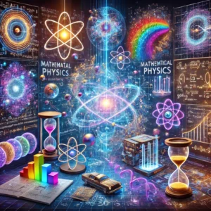
This illustration presents mathematical physics as a meeting place between abstract form and physical reality. At the center, luminous atomic-style rings and a radiant core suggest fundamental laws—symmetry, quantisation, and the deep “geometry” behind nature. Around them, chalkboard-like panels show equations, graphs, and diagrams, hinting at the tools of the field: calculus and differential equations for change, linear algebra for states and transformations, and complex analysis for waves, fields, and resonance. The scattered objects—books, measuring instruments, and twin hourglasses—evoke both study and experiment, reminding viewers that mathematical physics is not only about symbols, but about time, prediction, and understanding what can be measured. The overall effect is a rich, cosmic “workbench” where mathematics is used to model motion, energy, probability, and spacetime—turning physical questions into solvable structures, and solutions back into insight about the universe.
Applied Mathematics – Overview
Provides the bridge between abstract mathematics and physical reality through rigorous mathematical modeling.
Mathematical Physics
Uses mathematical structures such as differential equations, operator theory, and geometry to describe fundamental laws of nature.
Engineering Mathematics
Applies physical models in engineering contexts to design, control, and analyze real-world technical systems.
Computational Mathematics
Enables numerical simulation and neural network modeling of physical phenomena when analytical solutions are intractable.
Operations Research
Applies mathematical optimization and decision models to streamline resource allocation across physical and industrial networks.
Core Concepts & Foundation of Mathematical Physics
Mathematical physics applies mathematical techniques and theories to explore, model, and solve physical problems. It focuses on the precise formulation of physical laws and the development of abstract concepts that describe the universe.
1. Quantum Mechanics and Wave Equations: Describes particle behavior at subatomic scales. It utilizes Hilbert spaces to represent quantum states, linear operators for observables, and Schrödinger's differential equation to model quantum wave function evolution. Quantized energy states emerge naturally as matrix eigenvalues.
2. Relativity and Spacetime Geometry: Formulates gravitational phenomena as geometric curvature. Special Relativity uses Lorentz transformations in 4D Minkowski spacetime, while General Relativity uses differential geometry, tensors, and geodesics to describe spacetime curvature around massive stellar objects.
3. Statistical Mechanics and Thermodynamics: Connects microscopic particle states to macroscopic observables. Using partition functions, Boltzmann distributions, and entropy equations, mathematical physics explains phase transitions, heat capacity, and quantum phenomena like Bose-Einstein condensation.
About This Interactive Simulator:
This simulator models Quantum Wave Mechanics by computing the probability density function \(|\Psi(x,t)|^2\) for a particle in a 1D Infinite Potential Well (Particle in a Box). Users can adjust the quantum energy state principal number (\(n\)) to observe wave nodes and standing wave probability distributions.
- Solid Blue Line: Quantum Wave Function Probability Density \(|\Psi(x)|^2\)
- Dashed Red Line: Quantized Energy Level Threshold Line
- Quantum Number Slider (\(n\)): Sets the quantum state (\(n = 1, 2, 3, 4\)); higher \(n\) values increase wave oscillation and nodal points
Mathematical Physics: Quantum Particle in a Box Simulator
Applications of Mathematical Physics
Mathematical physics provides the theoretical rigor for modeling multi-scale phenomena across physical and technological domains:
1. Quantum Systems & Computing: Formulating quantum error-correction algorithms, quantum state tomography, and modeling electron transport in nanoscale semiconductors.
2. Gravitational Waves & Black Holes: Solving Einstein's non-linear field equations numerically to model binary black hole mergers and analyze gravitational wave signals detected by LIGO.
3. Plasma Physics & Astrophysics: Applying magnetohydrodynamics (MHD) and Navier-Stokes equations to simulate solar wind dynamics, accretion disks, and magnetic confinement in fusion reactors.
4. Condensed Matter Physics: Modeling topological insulators, electron band structures in graphene, and superfluid phase transitions using quantum field theory.
5. Physics-Informed AI & Neural Operators: Integrating mathematical physics laws (such as Fourier Neural Operators and PINNs) directly into deep learning architectures to discover conservation equations and accelerate simulations.
Emerging Trends, Challenges & Future Directions
Theoretical physics continues to push mathematical frontiers:
Emerging Trends:
- Quantum Information & Computing: Developing mathematical frameworks to optimize quantum circuits and simulate quantum many-body systems.
- String Theory & Quantum Gravity: Utilizing algebraic geometry and differential topology to unify general relativity with quantum field theory.
- Nonlinear Dynamics & Chaos: Analyzing non-linear differential equations governing fluid turbulence, climate systems, and chaotic orbits.
- Machine Learning in Physics: Training physics-informed neural networks (PINNs) to discover conservation laws and accelerate multi-scale simulations.
Key Challenges:
- Model Complexity: Reconciling non-linear physical formulations with rigorous analytical proofs.
- Computational Demands: Simulating high-dimensional quantum states and curved spacetime metrics requires petascale computing clusters.
Why Study Mathematical Physics?
Studying mathematical physics develops superior analytical reasoning, abstract problem-solving, and computational fluency, preparing graduates for cutting-edge research in quantum technology, astrophysics, data science, and quantitative modeling.
🎯 Career Guidance Tool Is Mathematical Physics Right For You?Explore career pathways, check your fit, and assess your skills — before you commit to a degree. | Explore Career Options → |
Frequently Asked Questions
What is Mathematical Physics and how does it differ from theoretical physics?
Mathematical Physics focuses on developing and using rigorous mathematical methods to formulate, analyse, and solve physical problems. The emphasis is on the structure of the equations, the properties of solutions, and the logical foundations of models. Theoretical physics is broader and often starts from physical intuition, building models that may initially be less rigorous. Mathematical physics lies at the interface: it sharpens physical ideas with precise mathematics and checks that models are internally consistent.
Why is Mathematical Physics important for students considering physics or engineering degrees?
Mathematical Physics trains students to move fluently between formulas and physical meaning. Topics such as differential equations, vector calculus, linear algebra, complex analysis, and variational principles appear in quantum mechanics, electromagnetism, fluid dynamics, and general relativity. A student who is comfortable with these tools can follow advanced lectures more easily, read research papers with confidence, and apply mathematics to new physical situations instead of memorising isolated formulas.
Which core mathematical topics are central to Mathematical Physics?
Key topics include ordinary and partial differential equations, vector calculus and tensor notation, complex numbers and complex analysis, linear algebra and eigenvalue problems, Fourier series and transforms, Green's functions, and basic functional analysis. These tools support major physical theories such as quantum mechanics, statistical mechanics, electromagnetism, and wave phenomena in optics and acoustics.
How are differential equations used in Mathematical Physics?
Differential equations describe how physical quantities change in space and time. In Mathematical Physics, students learn how Newton's laws, Maxwell's equations, the Schrödinger equation, and the heat and wave equations can all be written as differential equations. Techniques such as separation of variables, Fourier methods, Green's functions, and numerical schemes are used to solve these equations and interpret the solutions in terms of energy, conservation laws, boundary conditions, and symmetry.
Where do Fourier series and Fourier transforms appear in physical problems?
Fourier series and Fourier transforms allow complicated waves or signals to be expressed as sums or integrals of simple sinusoidal components. In Mathematical Physics, they are used to solve the heat and wave equations, to treat vibrating strings and membranes, to analyse diffraction and interference in optics, and to study quantum states in momentum space. They also form the mathematical basis of many modern technologies, including signal processing, image compression, and spectral analysis in laboratories.
How does linear algebra support topics such as quantum mechanics and normal modes?
Linear algebra provides the language of vectors, matrices, eigenvalues, and eigenvectors. In quantum mechanics, states are represented by vectors in a Hilbert space and physical observables by linear operators; eigenvalues represent measurable quantities such as energy. In classical physics, eigenvalue problems describe normal modes of coupled oscillators, vibrations of structures, and stability analysis. Mathematical Physics emphasises how these abstract concepts translate into concrete predictions about spectra, resonance, and time evolution.
What kinds of careers can benefit from a strong background in Mathematical Physics?
Graduates with training in Mathematical Physics are well prepared for research in physics and engineering, but their skills are also valuable in data science, quantitative finance, climate modelling, medical imaging, AI research, and high-tech industries. Employers value the ability to build models, analyse complex systems, and use both analytical and numerical methods. The combination of deep mathematical reasoning and physical intuition helps graduates tackle unfamiliar technical problems with confidence.
How can I study Mathematical Physics effectively at pre-university level?
A good strategy is to keep mathematics and physics closely connected. When you learn a new mathematical method, immediately look for physical examples where it applies—such as using differential equations for simple harmonic motion or exponential decay. Draw diagrams, track units carefully, and ask what each symbol represents physically. Work through fully solved examples, then try to adapt the method to new problems with slightly different boundary conditions or parameters. Using graphing tools or simple code to visualise solutions can also deepen understanding.
Comprehensive Practice & Knowledge Self-Assessment Module
Section 1: Foundational Review Questions & Answers
- How does Hilbert space structure quantum mechanical states? Answer: A Hilbert space is an abstract complex vector space with an inner product, providing the mathematical framework where quantum state vectors reside and self-adjoint operators represent observable physical quantities.
- What is the physical meaning of Schrödinger's time-dependent wave equation? Answer: It is a partial differential equation describing how the quantum wave function \(\Psi(x,t)\) evolves over time, where \(|\Psi(x,t)|^2\) determines the probability density of finding a particle at a given spatial coordinate.
- What role do geodesics play in General Relativity? Answer: Geodesics represent the extremum paths (shortest or longest intervals) through curved 4D spacetime, modeling the motion of freely falling particles under gravity without external forces.
- How does the partition function connect microstates to macroscopic thermodynamics? Answer: The partition function \(Z\) sums Boltzmann factors \(e^{-\beta E_i}\) over all microstates, allowing macroscopic thermodynamic properties like free energy, entropy, and pressure to be derived directly.
- What is the mathematical significance of Noether's Theorem? Answer: Noether's Theorem proves that every continuous differentiable symmetry of a physical action corresponds to a conserved physical quantity (e.g., time translation symmetry yields energy conservation).
- Why are partial differential equations essential in electrodynamics? Answer: Maxwell's equations are vector PDEs relating spatial derivatives (curl and divergence) of electric and magnetic fields to local charge and current densities.
- How does Fourier analysis resolve heat distribution problems? Answer: It decomposes arbitrary initial temperature distributions into orthogonal sinusoidal boundary modes that decay exponentially over time at rate proportional to their spatial frequency squared.
- What is the definition of a tensor in General Relativity? Answer: A tensor is a multi-linear geometric object that transforms predictably under coordinate conversions, ensuring physical laws remain invariant across arbitrary reference frames.
Section 2: Analytical & Thought-Provoking Questions
- How does the spectral theorem guarantee real physical measurements in quantum mechanics? Answer: The spectral theorem establishes that self-adjoint (Hermitian) operators in Hilbert space possess strictly real eigenvalues, ensuring physical observables like energy or momentum yield real scalar values upon measurement.
- Why do curvature singularities in General Relativity indicate mathematical limits of the theory? Answer: Infinite scalar curvature values (e.g., inside black holes) signal points where smooth Riemannian manifold metrics break down, necessitating a non-perturbative quantum gravity formulation.
- How does topological quantisation explain discrete magnetic flux in superconductors? Answer: Single-valued wave function phase continuity around a superconducting loop constrains phase changes to integer multiples of \(2\pi\), quantizing enclosed magnetic flux in exact units \(h / (2e)\).
- In what ways do non-linear differential equations generate chaotic dynamics in classical physics? Answer: Non-linear coupling terms create sensitive dependence on initial conditions (butterfly effect), where phase space trajectories diverge exponentially (positive Lyapunov exponents) within bounded attractors.
- How does group theory classify fundamental particles in quantum field theory? Answer: Fundamental particles correspond to irreducible representations of spacetime symmetry groups (Poincaré group) and internal gauge symmetry groups like \(\text{SU}(3) \times \text{SU}(2) \times \text{U}(1)\).
- Why is the mathematical formulation of quantum mechanics incompatible with classical general relativity? Answer: Quantum mechanics relies on a fixed background spacetime lattice for linear operator superposition, whereas General Relativity treats spacetime itself as a dynamic, non-linear physical variable.
- How does the ergodic hypothesis justify calculating time averages via ensemble averages in statistical mechanics? Answer: It posits that over long timescales, a microcanonical system's trajectory explores all accessible points in constant-energy phase space with equal probability, equating temporal and statistical averages.
Section 3: Numerical Problems & Solutions
Key Formula Callout: 1D Particle in a Box Quantum Energy Levels
$$E_n = \frac{n^2 \pi^2 \hbar^2}{2 m L^2} \qquad \Big| \qquad \Psi_n(x) = \sqrt{\frac{2}{L}} \sin\left(\frac{n \pi x}{L}\right)$$
Approximate \(I = \int_{0}^{\pi} \sin(x)\,dx\) using Simpson's Rule with \(n = 4\) subintervals.
Step size: \(h = \frac{\pi - 0}{4} = \frac{\pi}{4}\).
Nodes: \(x_0 = 0\), \(x_1 = \frac{\pi}{4}\), \(x_2 = \frac{\pi}{2}\), \(x_3 = \frac{3\pi}{4}\), \(x_4 = \pi\).
Evaluating \(f(x) = \sin(x)\):
\(f(0) = 0\), \(f\left(\frac{\pi}{4}\right) = \frac{\sqrt{2}}{2} \approx 0.7071\), \(f\left(\frac{\pi}{2}\right) = 1.0\), \(f\left(\frac{3\pi}{4}\right) = \frac{\sqrt{2}}{2} \approx 0.7071\), \(f(\pi) = 0\).
Simpson's Formula: $$S = \frac{h}{3} \left[ f(x_0) + f(x_4) + 4\left(f(x_1) + f(x_3)\right) + 2 f(x_2) \right]$$ $$S = \frac{\pi}{12} \left[ 0 + 0 + 4(0.7071 + 0.7071) + 2(1.0) \right] = \frac{\pi}{12} \left[ 4(1.4142) + 2.0 \right]$$ $$S = \frac{\pi}{12} [5.6568 + 2.0] = \frac{\pi}{12} \times 7.6568 \approx 2.0045$$
Find the root of \(f(x) = x^2 - 3 = 0\) starting from \(x_0 = 2.0\).
Derivative: \(f'(x) = 2x\).
Iteration 1: $$x_1 = x_0 - \frac{f(x_0)}{f'(x_0)} = 2.0 - \frac{4 - 3}{4.0} = 2.0 - 0.25 = 1.75$$ Iteration 2: $$f(1.75) = (1.75)^2 - 3 = 3.0625 - 3 = 0.0625$$ $$f'(1.75) = 2(1.75) = 3.5$$ $$x_2 = 1.75 - \frac{0.0625}{3.5} = 1.75 - 0.01786 = 1.73214$$ (Approximating \(\sqrt{3} \approx 1.73205\)).
Estimate \(f'(1)\) for \(f(x) = e^x\) with step size \(h = 0.01\).
Formula: $$f'(1) \approx \frac{f(1 + h) - f(1)}{h}$$ \(f(1) = e^1 \approx 2.71828\).
\(f(1.01) = e^{1.01} \approx 2.74560\).
$$\text{Approximation} = \frac{2.74560 - 2.71828}{0.01} = 2.7320$$ Truncation error \(= |2.7320 - 2.71828| = 0.01372\) (bounded by \(\frac{h}{2} f''(1) \approx 0.005 \times 2.718 = 0.0136\)).
Perform 1 iteration for system \(3x + y = 10\), \(x + 4y = 11\) starting from \((x_0, y_0) = (2, 2)\).
Rearrange equations: $$x = \frac{10 - y}{3}$$ $$y = \frac{11 - x}{4}$$ Update \(x_1\): $$x_1 = \frac{10 - 2}{3} = \frac{8}{3} \approx 2.6667$$ Update \(y_1\) using updated \(x_1\): $$y_1 = \frac{11 - 2.6667}{4} = \frac{8.3333}{4} \approx 2.0833$$ First iteration values: \((x_1, y_1) = (2.6667, 2.0833)\).
Find the characteristic polynomial and eigenvalues of \(\mathbf{A} = \begin{pmatrix} 4 & 1 & 0 \\ 1 & 3 & 1 \\ 0 & 1 & 2 \end{pmatrix}\).
Characteristic equation: \(\det(\mathbf{A} - \lambda\mathbf{I}) = 0\). $$\det \begin{pmatrix} 4 - \lambda & 1 & 0 \\ 1 & 3 - \lambda & 1 \\ 0 & 1 & 2 - \lambda \end{pmatrix} = 0$$ Expanding along top row: $$(4 - \lambda) \left[(3 - \lambda)(2 - \lambda) - 1\right] - 1 \left[(1)(2 - \lambda) - 0\right] = 0$$ $$(4 - \lambda) [\lambda^2 - 5\lambda + 5] - (2 - \lambda) = 0$$ $$(4\lambda^2 - 20\lambda + 20 - \lambda^3 + 5\lambda^2 - 5\lambda) - 2 + \lambda = 0$$ $$-\lambda^3 + 9\lambda^2 - 24\lambda + 18 = 0 \Rightarrow \lambda^3 - 9\lambda^2 + 24\lambda - 18 = 0$$ Factoring: $$(\lambda - 3)(\lambda^2 - 6\lambda + 6) = 0$$ Eigenvalues: \(\lambda_1 = 3\), and roots of \(\lambda^2 - 6\lambda + 6 = 0\): $$\lambda = \frac{6 \pm \sqrt{12}}{2} = 3 \pm \sqrt{3}$$ Eigenvalues are \(\lambda = 3\), \(3 + \sqrt{3} \approx 4.732\), and \(3 - \sqrt{3} \approx 1.268\).
Find \(f'(2)\) for \(f(x) = \ln(x)\) using central differences with \(h = 0.01\).
Formula: $$f'(x) \approx \frac{f(x + h) - f(x - h)}{2h}$$ \(f(2.01) = \ln(2.01) \approx 0.698135\).
\(f(1.99) = \ln(1.99) \approx 0.688135\).
$$\text{Approximation} = \frac{0.698135 - 0.688135}{0.02} = \frac{0.010000}{0.02} = 0.5000$$ (Exact analytical derivative \(\frac{1}{x}\) at \(x = 2\) is \(0.5\); central differences eliminate \(\mathcal{O}(h)\) error terms).
Solve \(\frac{dy}{dx} = x - y\), \(y(0) = 1\) for 1 step with \(h = 0.1\).
\(f(x, y) = x - y\); \(x_0 = 0\), \(y_0 = 1\), \(h = 0.1\).
$$k_1 = f(0, 1) = 0 - 1 = -1.0$$ $$k_2 = f(0 + 0.05, 1 + 0.05(-1.0)) = f(0.05, 0.95) = 0.05 - 0.95 = -0.90$$ $$k_3 = f(0 + 0.05, 1 + 0.05(-0.90)) = f(0.05, 0.955) = 0.05 - 0.955 = -0.905$$ $$k_4 = f(0 + 0.1, 1 + 0.1(-0.905)) = f(0.1, 0.9095) = 0.1 - 0.9095 = -0.8095$$ $$y_1 = y_0 + \frac{h}{6} [k_1 + 2k_2 + 2k_3 + k_4]$$ $$\text{Sum} = -1.0 + 2(-0.90) + 2(-0.905) - 0.8095 = -1.0 - 1.80 - 1.81 - 0.8095 = -5.4195$$ $$y_1 = 1 + \left(\frac{0.1}{6}\right) \times (-5.4195) = 1 - 0.090325 = 0.909675$$