
Computational mathematics is the engine that drives much of modern science, engineering, and finance. In the artificial intelligence era, it provides the fundamental numerical algorithms that power machine learning optimizers, neural operators, high-dimensional tensor calculations, and scientific surrogate modeling. Building on the core principles of mathematics, it blends theoretical insight with numerical methods to solve problems that are too complex for analytical solutions. Whether modeling financial products in actuarial science or optimizing assets in investment and portfolio management, the power of computation allows practitioners to simulate uncertainty and evaluate risk with speed and precision.
Students entering fields like life insurance and pension systems will find that computational approaches are essential for pricing policies, forecasting liabilities, and managing long-term solvency. These same tools are equally valuable in applied mathematics, where they support real-world modeling in physics, computational biology, epidemiological forecasting, and engineering systems.
Specialized areas such as engineering mathematics and mathematical physics frequently depend on computational solutions for complex differential equations, dynamic systems, and simulations of physical phenomena. Modern scientific computing increasingly merges these formulations with physics-informed neural networks (PINNs) and deep operator networks to accelerate multi-scale discoveries. Likewise, decision-making processes in logistics and infrastructure are powered by methods found in operations research, where computing efficiency is vital to real-time analytics and optimization.
Computational mathematics is inseparable from its theoretical roots in pure mathematics. Concepts from algebra, calculus, and mathematical analysis form the basis for algorithms, stability proofs, and discrete numerical schemes. Moreover, insights from geometry, topology, and number theory are increasingly relevant in areas like topological data analysis, image processing, post-quantum cryptography, and neural network loss landscape analysis.
As data becomes central to all industries, the role of statistics and computation continues to grow. Through descriptive statistics and inferential statistics, computational methods enable insights into vast datasets and support machine learning algorithms that transform how we understand patterns, assess parameter sensitivities, and generate predictive distributions.
Beyond mathematics, computational tools are crucial in developing emerging technologies. In physical technologies, simulations are used to test and design cutting-edge systems. Aerospace fields, such as aerospace and aeronautical engineering, rely on complex models of fluid dynamics, materials behavior, and control systems. Subfields like aero control systems and robotics and aero materials science showcase how computation allows for precise modeling and real-time control. Mastering computational mathematics thus equips students with a universal skill set adaptable to scientific computing, artificial intelligence, quantitative finance, and industrial engineering.
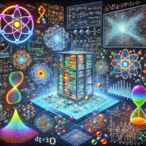
This illustration places a luminous computing core—shown as a server stack—at the center of a digital “workbench,” implying that modern mathematics is often executed, tested, and refined through computation. Around it float chalkboard-style formulas, plotted curves, network diagrams, and abstract scientific motifs (atoms, fractal spirals, and waveform graphs), representing numerical methods, optimisation, and large-scale modelling. The hourglass and time-step cue hint at iterative algorithms and simulations that evolve step by step, such as solving differential equations, running Monte Carlo experiments, or training numerical solvers. Overall, the image conveys computational mathematics as the bridge between pure theory and real-world calculation—using algorithms, code, and high-performance computing to approximate, visualise, and verify complex mathematical ideas.
Applied Mathematics – Overview
Establishes how mathematical theory is translated into practical computational applications across science, engineering, and logistics.
Computational Mathematics
Develops numerical methods and algorithms to approximate solutions for complex problems that cannot be solved analytically.
Engineering Mathematics
Supplies governing equations that computational methods solve through finite elements, transforms, and numerical approximation.
Mathematical Physics
Provides complex physical models that require high-performance computational techniques for simulation and predictive modeling.
Operations Research
Uses computational algorithms to solve large-scale optimization, linear programming, and scheduling problems efficiently.
Core Concepts & Key Domains in Computational Mathematics
Computational mathematics focuses on creating and implementing computational algorithms, numerical methods, and models to solve mathematical problems that require extensive computations. It addresses challenges ranging from large-scale simulations to data-driven insights in artificial intelligence, offering tools to study systems in fields like physics, biology, and finance.
1. Numerical Analysis: Involves designing and analyzing algorithms to approximate solutions for mathematical problems, especially those involving differential equations, linear algebra, and optimization. Key techniques include root-finding algorithms (e.g., Newton's method, bisection method), numerical integration/differentiation, and the Finite Element Method (FEM) used for stress analysis in structural engineering and fluid flow simulation in aerodynamics.
2. High-Performance Computing (HPC): Utilizes supercomputers and parallel processing to solve massive, computationally intensive problems. By leveraging cluster computing and parallel task distribution, HPC enables climate models for global warming forecasts, biological simulations of protein folding, and astronomical predictions of galactic movement.
3. Algorithm Development: Focuses on engineering efficient, mathematically optimized algorithms. This includes machine learning structures (neural networks, decision trees), graph algorithms for logistics and social network analysis, and cryptographic protocols (RSA, ECC, hashing) vital for securing communication and blockchain networks.
4. Computational Modeling and Simulation: Constructs digital representations of physical and probabilistic systems. Techniques like Monte Carlo simulations use random sampling to evaluate financial risk and drug discovery, agent-based models simulate urban traffic flow, and multiscale modeling bridges chemical reactions from molecular to macroscopic levels.
About This Interactive Simulator:
This simulator demonstrates the convergence behavior and iteration speed of the Newton-Raphson numerical root-finding algorithm. Users can adjust the initial guess (\(x_0\)) and target precision iteration steps to visualize how iterative tangent lines converge toward function zeroes.
- Solid Blue Line: Continuous Function Curve \(f(x) = x^2 - 2\)
- Dashed Red Line: Tangent secant projection drawn during iteration \(k\)
- Initial Guess Slider (\(x_0\)): Adjusts starting value to examine convergence rate and numerical stability
Computational Mathematics: Newton-Raphson Root-Finding Simulator
Applications of Computational Mathematics
Computational mathematics forms the computational backbone across multidisciplinary industrial and scientific domains:
1. Climate Science: Simulating atmospheric dynamics, ocean circulation, and carbon sequestration models using partial differential equations to forecast global climate trends and hurricane paths.
2. Cryptography and Cybersecurity: Developing public-key encryption architectures (RSA, Elliptic Curve Cryptography) and post-quantum lattice protocols to secure digital transactions and decentralized blockchain ledgers.
3. Drug Discovery & Molecular Biology: Modeling molecular docking and protein-ligand interactions via Monte Carlo and molecular dynamics techniques to evaluate candidate efficacy prior to chemical synthesis.
4. Artificial Intelligence & Machine Learning: Utilizing stochastic gradient descent optimization, high-dimensional tensor operations, and probabilistic modeling to train deep neural networks for scientific machine learning and algorithmic systems.
5. Computational Fluid Dynamics (CFD): Solving Navier-Stokes equations to optimize aerodynamic drag on aircraft wings, automotive structures, and coolant flow within nuclear power systems.
Emerging Trends, Challenges & Future Directions
As computing infrastructure transforms, computational mathematics continues to push modern frontiers:
Emerging Trends:
- Quantum Computing & Quantum Numerical Linear Algebra: Designing quantum algorithms (such as HHL) to tackle matrix inversion, high-dimensional linear systems, and molecular state simulations exponentially faster than classical supercomputers.
- Physics-Informed Neural Networks (PINNs): Merging scientific machine learning with differential equation solvers to embed conservation laws directly into neural loss functions.
- Multiphysics Simulations & Digital Twins: Coupling simultaneous thermal, structural, and fluid dynamic interactions within real-time predictive digital twin environments.
Challenges in the Field:
- Computational Complexity & High Dimensionality: High-dimensional optimization and continuous state spaces demand massive parallel memory bandwidth and processor scaling.
- Numerical Stability & Error Control: Bounding cumulative round-off errors and guaranteeing algorithmic convergence across stiff, highly non-linear physical systems.
Why Study Computational Mathematics?
Combining mathematical rigor with programming fluency equips students with highly sought-after competencies across scientific computing, AI development, data science, quantitative finance, and aerospace engineering.
🎯 Career Guidance Tool Is Computational Mathematics Right For You?Explore career pathways, check your fit, and assess your skills — before you commit to a degree. | Explore Career Options → |
Frequently Asked Questions
What is computational mathematics?
Computational mathematics is the study of numerical methods, algorithms, and computer-based techniques used to solve mathematical problems that are difficult or impossible to handle with algebraic methods alone. It combines ideas from applied mathematics, numerical analysis, and computer science.
How is computational mathematics different from pure and applied mathematics?
Pure mathematics focuses on theory and proofs, while applied mathematics builds models for real-world problems. Computational mathematics sits alongside them and focuses on how to turn these models into algorithms that a computer can run efficiently and accurately.
Do I need strong programming skills before studying computational mathematics?
You do not need to be an expert programmer to start, but you should be willing to learn at least one programming language such as Python, MATLAB, or Julia. Over time, your coding skills will develop as you implement algorithms, run simulations, and analyse numerical results.
What school topics help me prepare for computational mathematics?
Strong foundations in algebra, functions, calculus, and vectors are very helpful. Exposure to basic statistics, matrices, and some introductory programming will also make it easier to understand numerical methods and algorithmic thinking later on.
What kinds of problems does computational mathematics solve?
Computational mathematics is used to solve large systems of equations, approximate solutions of differential equations, optimise complex systems, simulate physical processes, and handle high-dimensional data. These problems often arise in engineering, finance, climate modelling, and many other fields.
Which software tools and languages are commonly used in computational mathematics?
Common tools include Python with scientific libraries such as NumPy and SciPy, MATLAB or Octave for numerical computing, and languages like Julia, C++, or R for more specialised tasks. Many students start with Python or MATLAB because they are widely used in universities and industry.
How is computational mathematics used in data science, AI, and engineering?
In data science and AI, computational mathematics underpins optimisation algorithms, numerical linear algebra, and probabilistic models used for training machine-learning systems. In engineering, it supports simulations of structures, fluids, materials, and control systems, allowing designers to test ideas before building real prototypes.
What career paths can knowledge of computational mathematics lead to?
Graduates with computational mathematics skills can work in areas such as scientific computing, quantitative finance, data science, engineering simulation, operations research, and software development. The combination of mathematical modelling and programming is highly valued across many technical careers.
Comprehensive Practice & Knowledge Self-Assessment Module
Section 1: Foundational Review Questions & Answers
- What defines computational mathematics as a distinct discipline? Answer: It bridges pure mathematics and computer science by developing algorithms, numerical approximations, and computer simulations to solve mathematical models that are too complex for analytical solutions.
- What is the core objective of numerical analysis? Answer: To design, evaluate, and implement algorithms for approximating solutions to continuous mathematical problems while quantifying and controlling truncation and round-off errors.
- How does high-performance computing (HPC) transform scientific research? Answer: HPC utilizes parallel computing and supercomputers to distribute complex matrix operations and large-scale grid simulations across thousands of processor cores simultaneously.
- What role do Monte Carlo simulations play in risk modeling? Answer: Monte Carlo methods rely on repeated random sampling to generate probability distributions for systems with significant inherent uncertainty, such as portfolio valuation or disease spread.
- Why are finite element methods (FEM) widely used in engineering? Answer: FEM subdivides complex physical structures into smaller, simpler finite elements to numerically approximate solutions for partial differential equations governing stress, heat transfer, and fluid dynamics.
- How does computational mathematics contribute to cryptography? Answer: It provides number-theoretic algorithms for prime factorization, discrete logarithms, and elliptic curve operations that form the backbone of modern digital encryption protocols.
- What is the function of gradient descent in artificial intelligence? Answer: Gradient descent is an iterative optimization algorithm used to minimize loss functions during neural network training by adjusting weight parameters along the negative gradient direction.
- Why are numerical software environments like MATLAB and Python scientific libraries essential? Answer: They provide optimized, high-level matrix manipulation libraries, differential equation solvers, and visualization tools that streamline algorithm implementation and rapid prototyping.
Section 2: Analytical & Thought-Provoking Questions
- How will the integration of quantum computing redefine numerical linear algebra algorithms? Answer: Quantum algorithms like HHL (Harrow-Hassidim-Lloyd) offer exponential speedups for solving linear systems \(A\mathbf{x} = \mathbf{b}\), potentially revolutionizing large-scale differential equation solvers and optimization routines.
- What trade-offs exist between numerical stability and computational speed in real-time simulations? Answer: Explicit numerical schemes are fast per time step but require strict stability step-size limits (Courant-Friedrichs-Lewy condition), whereas implicit schemes are unconditionally stable but require costly matrix inversions at each step.
- How do physics-informed neural networks (PINNs) challenge traditional finite element methods? Answer: PINNs incorporate partial differential equation residual terms directly into the loss function, allowing neural networks to solve forward and inverse physical problems without explicit mesh generation.
- In what ways can numerical round-off error accumulate to destabilize long-term scientific simulations? Answer: Floating-point arithmetic limits precision; across millions of iterative calculations, small round-off inaccuracies can compound exponentially, leading to numerical drift or catastrophic cancellation.
- How does agent-based modeling complement traditional differential equations in epidemiology? Answer: While differential equations model population-level averages, agent-based models simulate individual autonomous agents, capturing granular spatial, behavioral, and demographic heterogeneities.
- What challenges arise when scaling computational fluid dynamics (CFD) to turbulent flow regimes? Answer: Turbulent flows exhibit multi-scale energy cascades requiring extremely fine spatial and temporal grids (Direct Numerical Simulation), leading to extreme computational cost that scales as \(\text{Re}^3\).
- How does uncertainty quantification (UQ) improve confidence in predictive computational models? Answer: UQ systematically propagates input parameter variations through computational solvers to establish statistical confidence intervals around model predictions, ensuring reliable decision-making under uncertainty.
Section 3: Numerical Problems & Solutions (LaTeX Formatted Derivations)
Key Formula Callout: Newton-Raphson Root Iteration
$$x_{k+1} = x_k - \frac{f(x_k)}{f'(x_k)}$$
Approximate \(I = \int_{0}^{\pi} \sin(x)\,dx\) using Simpson's Rule with \(n = 4\) subintervals.
Step size: \(h = \frac{\pi - 0}{4} = \frac{\pi}{4}\).
Nodes: \(x_0 = 0\), \(x_1 = \frac{\pi}{4}\), \(x_2 = \frac{\pi}{2}\), \(x_3 = \frac{3\pi}{4}\), \(x_4 = \pi\).
Evaluating \(f(x) = \sin(x)\):
\(f(0) = 0\), \(f\left(\frac{\pi}{4}\right) = \frac{\sqrt{2}}{2} \approx 0.7071\), \(f\left(\frac{\pi}{2}\right) = 1.0\), \(f\left(\frac{3\pi}{4}\right) = \frac{\sqrt{2}}{2} \approx 0.7071\), \(f(\pi) = 0\).
Simpson's Formula: $$S = \frac{h}{3} \left[ f(x_0) + f(x_4) + 4\left(f(x_1) + f(x_3)\right) + 2 f(x_2) \right]$$ $$S = \frac{\pi}{12} \left[ 0 + 0 + 4(0.7071 + 0.7071) + 2(1.0) \right] = \frac{\pi}{12} \left[ 4(1.4142) + 2.0 \right]$$ $$S = \frac{\pi}{12} [5.6568 + 2.0] = \frac{\pi}{12} \times 7.6568 \approx 2.0045$$
Find the approximation for \(\sqrt{2}\) by solving \(f(x) = x^2 - 2 = 0\) with initial guess \(x_0 = 1.5\).
Derivative: \(f'(x) = 2x\).
Iteration 1: $$x_1 = x_0 - \frac{f(x_0)}{f'(x_0)} = 1.5 - \frac{(1.5)^2 - 2}{2(1.5)} = 1.5 - \frac{2.25 - 2}{3.0} = 1.5 - \frac{0.25}{3.0} = 1.5 - 0.08333 = 1.41667$$ Iteration 2: $$f(1.41667) = (1.41667)^2 - 2 = 2.00694 - 2 = 0.00694$$ $$f'(1.41667) = 2(1.41667) = 2.83334$$ $$x_2 = 1.41667 - \frac{0.00694}{2.83334} = 1.41667 - 0.00245 = 1.41422$$ (Accurate to 4 decimal places of \(\sqrt{2} \approx 1.41421\)).
Estimate \(f'(1)\) for \(f(x) = e^x\) using the forward difference formula with step size \(h = 0.01\).
Forward difference formula: $$f'(x) \approx \frac{f(x + h) - f(x)}{h}$$ Evaluate points: \(f(1) = e^1 \approx 2.71828\), \(f(1.01) = e^{1.01} \approx 2.74560\).
$$f'(1) \approx \frac{2.74560 - 2.71828}{0.01} = \frac{0.02732}{0.01} = 2.7320$$ Exact analytical value: \(f'(1) = e^1 \approx 2.71828\).
Absolute truncation error \(= |2.7320 - 2.71828| = 0.01372\).
Theoretical leading error bound: $$\text{Error} \approx \frac{h}{2} f''(\xi) \approx \frac{0.01}{2} \times 2.718 \approx 0.0136$$
Perform 1 iteration of Gauss-Seidel for \(4x + y = 9\), \(x + 3y = 8\), starting with \((x_0, y_0) = (1, 1)\).
Rearrange equations in diagonally dominant fixed-point form: $$x = \frac{9 - y}{4}$$ $$y = \frac{8 - x}{3}$$ Update \(x_1\): $$x_1 = \frac{9 - y_0}{4} = \frac{9 - 1}{4} = \frac{8}{4} = 2.0$$ Update \(y_1\) using the updated value \(x_1\): $$y_1 = \frac{8 - x_1}{3} = \frac{8 - 2.0}{3} = \frac{6}{3} = 2.0$$ After 1 iteration, \((x_1, y_1) = (2.0, 2.0)\).
Solve \(\frac{dy}{dx} = x + y\), \(y(0) = 1\) for 1 step with \(h = 0.1\).
Given \(f(x, y) = x + y\), \(x_0 = 0\), \(y_0 = 1\), \(h = 0.1\): $$k_1 = f(0, 1) = 0 + 1 = 1.0$$ $$k_2 = f(0 + 0.05, 1 + 0.05 \times 1.0) = f(0.05, 1.05) = 0.05 + 1.05 = 1.10$$ $$k_3 = f(0 + 0.05, 1 + 0.05 \times 1.10) = f(0.05, 1.055) = 0.05 + 1.055 = 1.105$$ $$k_4 = f(0 + 0.1, 1 + 0.1 \times 1.105) = f(0.1, 1.1105) = 0.1 + 1.1105 = 1.2105$$ Weighted summation: $$\sum k = k_1 + 2k_2 + 2k_3 + k_4 = 1.0 + 2(1.10) + 2(1.105) + 1.2105 = 6.6205$$ $$y_1 = y_0 + \frac{h}{6} \sum k = 1 + \frac{0.1}{6}(6.6205) = 1 + 0.11034 = 1.11034$$ The numerical approximation for \(y(0.1)\) is \(1.11034\).
Estimate \(I = \int_{0}^{1} x\,dx\) using 4 random uniform evaluation points: \(U = \{0.1, 0.3, 0.6, 0.8\}\).
Evaluate \(f(U_i) = U_i\):
\(f(0.1) = 0.1\), \(f(0.3) = 0.3\), \(f(0.6) = 0.6\), \(f(0.8) = 0.8\).
Monte Carlo integration formula: $$I \approx \frac{1}{N} \sum_{i=1}^{N} f(U_i) = \frac{0.1 + 0.3 + 0.6 + 0.8}{4} = \frac{1.8}{4} = 0.45$$ Analytical Comparison: The exact analytical integral is \(\int_{0}^{1} x\,dx = \left[\frac{x^2}{2}\right]_0^1 = 0.5\). The empirical estimate converges toward \(0.5\) as \(N \to \infty\).
Test fixed-point iteration \(x_{k+1} = \cos(x_k)\) starting from initial estimate \(x_0 = 0.5\) for 2 steps.
Step 1: $$x_1 = \cos(0.5) \approx 0.87758$$ Step 2: $$x_2 = \cos(0.87758) \approx 0.63901$$ Successive step difference: $$|x_2 - x_1| = |0.63901 - 0.87758| = 0.23857$$ The iteration oscillates while converging toward the unique Dottie number fixed point (\(x \approx 0.73908\)).