
Interactive Quick Review: Exact KNN vs. Approximate ANN Search
Why are production vector databases built around Approximate Nearest Neighbor (ANN) search rather than exact k-Nearest Neighbors (kNN)?
Toggle Answer
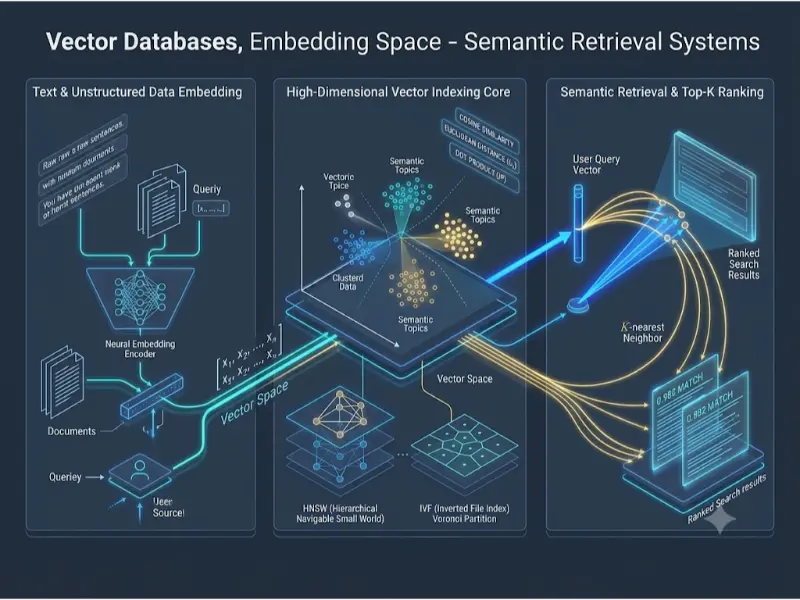
Answer: Exact kNN requires computing distance metrics between a query vector and every single vector in the database, resulting in linear computational complexity O(N · d). Over millions of 1536-dimensional vectors, exact scanning takes seconds per query. ANN algorithms (like HNSW or IVF) build spatial index graphs that reduce search time to O(log N), answering queries in sub-10 milliseconds with >95% recall accuracy.
Architectural & Theoretical Deep Dives
1. Vector Distance & Similarity Metrics
The foundation of vector retrieval is measuring proximity between query vector u and document vector v in d-dimensional continuous space Rd:
- Cosine Similarity: Measures the angle between two vectors, ignoring vector magnitude. Highly effective for normalized text embeddings:
$$\text{CosineSimilarity}(\mathbf{u}, \mathbf{v}) = \frac{\mathbf{u} \cdot \mathbf{v}}{\|\mathbf{u}\| \|\mathbf{v}\|} = \frac{\sum_{i=1}^d u_i v_i}{\sqrt{\sum_{i=1}^d u_i^2} \sqrt{\sum_{i=1}^d v_i^2}}$$
- Dot Product (Inner Product – IP): Measures both angle and vector magnitude. When vectors are L2-normalized (||u|| = ||v|| = 1), Dot Product is mathematically identical to Cosine Similarity but requires fewer GPU floating-point operations:
$$\text{DotProduct}(\mathbf{u}, \mathbf{v}) = \mathbf{u} \cdot \mathbf{v} = \sum_{i=1}^d u_i v_i$$
- Euclidean Distance (L2 Norm): Measures straight-line spatial distance between coordinate endpoints. Smaller values indicate higher similarity:
$$d_{L_2}(\mathbf{u}, \mathbf{v}) = \|\mathbf{u} – \mathbf{v}\|_2 = \sqrt{\sum_{i=1}^d (u_i – v_i)^2}$$
2. ANN Indexing Strategies: HNSW and IVF
Vector databases organize continuous space using specialized indexing algorithms:
Hierarchical Navigable Small World (HNSW): A multi-layer graph index. Top layers contain sparse, long-range connections for fast highway routing across vector space. Lower layers contain dense, short-range connections for granular nearest-neighbor convergence. HNSW delivers ultra-low search latency and high recall, but consumes significant RAM memory.
Inverted File Index (IVF): Partitions vector space into C Voronoi cells using k-means clustering. During retrieval, the query vector is assigned to its nearest cluster centroids, and search is restricted purely to vectors inside those active Voronoi cells, reducing comparison operations by 90%+.
3. Vector Quantization: Product Quantization (PQ) & Scalar Quantization (SQ)
Storing high-dimensional float32 vectors in RAM creates immense memory costs (a 1B vector dataset at d = 1536 requires 6 TB of memory). Databases compress vectors using quantization:
- Scalar Quantization (SQ8): Converts 32-bit floating-point coordinates into 8-bit integers (int8), reducing RAM consumption by 75% with minimal recall degradation.
- Product Quantization (PQ): Divides a d-dimensional vector into m smaller sub-vectors, maps each sub-vector to its nearest codebook centroid, and stores centroid index IDs instead of raw numbers, achieving compression ratios up to 95%+.
4. Python Implementation: HNSW Indexing & Cosine Search with FAISS
import numpy as np

import faiss


# 1. Setup Dataset and Dimensions

dimension = 128         # Embedding dimension

num_vectors = 10000     # Size of vector database index

num_queries = 2         # Search queries


np.random.seed(42)

# Generate dummy normalized float32 vectors

db_vectors = np.random.randn(num_vectors, dimension).astype('float32')

faiss.normalize_L2(db_vectors) # Normalize for inner product == cosine similarity


query_vectors = np.random.randn(num_queries, dimension).astype('float32')

faiss.normalize_L2(query_vectors)


# 2. Build HNSW Index (M=16 connections per node, Inner Product metric)

M = 16

index = faiss.IndexHNSWFlat(dimension, M, faiss.METRIC_INNER_PRODUCT)

index.hnsw.efConstruction = 64 # Construction accuracy parameter


# Add vectors to index

index.add(db_vectors)

print(f"Total Vectors Indexed: {index.ntotal}")


# 3. Perform ANN Search (Top-K = 3 nearest neighbors)

k = 3

index.hnsw.efSearch = 32 # Runtime search accuracy parameter

distances, indices = index.search(query_vectors, k)


# Output Results

for q_idx in range(num_queries):

    print(f"\n--- Query {q_idx + 1} Results ---")

    for rank in range(k):

        doc_id = indices[q_idx][rank]

        cosine_score = distances[q_idx][rank]

        print(f"Rank {rank + 1}: Doc ID = {doc_id}, Cosine Score = {cosine_score:.4f}")
Interactive Quick Review: Dense Semantic vs. Sparse Keyword Indexing
When should a retrieval system use dense vector embeddings versus sparse inverted indexes (BM25)?
Toggle Answer
Answer: Dense Vector Search excels at understanding intent, synonyms, concept matching, and cross-lingual queries where exact wording differs. Sparse BM25 Search excels at exact keyword matching, technical part numbers, acronyms, and rare proper nouns. Modern architectures use Hybrid Search (fusing both dense vector and sparse keyword scores via Reciprocal Rank Fusion) to achieve optimal retrieval across all query types.
Taxonomy & Index Optimization Matrix
| ANN Index Type | Mechanism | Search Latency | RAM Memory Footprint | Index Build Time |
|---|---|---|---|---|
| Flat Index (Exact kNN) | Brute-force distance scan over raw vectors | Very High (O(N)) | Baseline (Raw vectors) | Zero (No index build) |
| HNSW (Hierarchical Graph) | Multi-layer small-world graph traversal | Ultra-Low (O(log N)) | Very High (Raw vectors + graph edges) | Slow / Memory intensive |
| IVF-Flat (Inverted File) | K-means Voronoi spatial clustering | Low (Searches targeted clusters) | Low-Moderate | Moderate (Requires centroid training) |
| IVF-PQ (Quantized IVF) | Voronoi clusters + Product Quantization | Low | Ultra-Low (Up to 95% compressed) | Slow (Centroid + Codebook training) |
Applications, Trade-offs, & Future Outlook
Real-World Applications
- Retrieval-Augmented Generation (RAG): Serving as the authoritative long-term memory store for grounding Large Language Models on enterprise document knowledge.
- Multimodal Media Search: Connecting CLIP-style text and image embeddings to allow natural language visual queries (e.g., searching “sunset over mountains” to retrieve matching un-tagged photos).
- E-Commerce Semantic Recommendations: Mapping user behavioral interactions and product catalogs into shared vector space to serve personalized product matches.
Engineering Trade-offs
The central dilemma in vector database architecture is the Recall vs. Latency vs. Memory Trilemma. Achieving >99% recall requires dense graph structures (HNSW) loaded entirely into expensive RAM. Quantizing vectors (PQ/SQ) or reducing M connection parameters lowers memory overhead dramatically, but risks dropping relevant document matches during high-concurrency retrieval.
Future Outlook & Emerging Research
State-of-the-art vector systems are moving toward Native Disk-Based ANN Indexing (e.g., DiskANN), using memory-mapped SSD storage combined with compressed RAM caches to serve billion-scale indices at fractional infrastructure costs. Concurrently, ColBERT multi-vector representations are bridging the gap between single-vector dense models and fine-grained token-level cross-attention.
Frequently Asked Questions
What is the difference between Vector Indexing and Vector Storage?
Vector Indexing refers to data structures (like HNSW graphs or IVF clusters) built to accelerate approximate nearest-neighbor search. Vector Storage refers to the underlying database engine responsible for persistence, metadata filtering, payload storage, ACID compliance, and distributed sharding.
Why is L2-normalization recommended before indexing vectors?
Normalizing vectors so their magnitude equals 1.0 (||v||2 = 1) makes Dot Product mathematically equivalent to Cosine Similarity. Computing Dot Product skips square root and division instructions, allowing hardware tensor cores to execute vector similarity math up to 3× faster.
What is Metadata Filtering in Vector Databases?
Metadata filtering restricts vector search results based on structured attributes (e.g., user_id == 104 or date > 2026-01-01). Modern databases perform Single-Pass Filtered Search during HNSW graph traversal to prevent orphaned graph branches or post-filtering result depletion.
What is the “Curse of Dimensionality” in Vector Space?
In high-dimensional spaces (e.g., d > 512), spatial volume grows exponentially, making all data points appear roughly equidistant from one another under standard Euclidean metrics. Neural embedding models solve this by structuring data into lower-dimensional continuous manifolds within high-dimensional space.
End-of-Page Exercises & Assessment
Part 1: Review Questions
Q1: Define a Dense Vector Embedding and explain how it differs from a Sparse One-Hot Vector.
Answer: A Dense Vector Embedding is a continuous array of real numbers (e.g., 1536 float32 values) where every coordinate contains non-zero latent information capturing semantic concepts. A Sparse One-Hot Vector is a high-dimensional discrete array (e.g., 100,000 vocabulary dimension) consisting almost entirely of zeros except for a single 1 at the specific word’s index.
Q2: What mathematical property holds when computing Dot Product on L2-normalized vectors?
Answer: For L2-normalized vectors (||u|| = ||v|| = 1), the Dot Product is mathematically equal to Cosine Similarity because the denominator ||u|| ||v|| = 1.
Q3: Explain the multi-layer structure of a Hierarchical Navigable Small World (HNSW) graph index.
Answer: Top layers contain sparse node connections with long-range links for rapid coarse routing across distant regions of vector space. Lower layers contain dense node connections with short-range links for fine-grained convergence to nearest neighbors.
Q4: How does Product Quantization (PQ) compress high-dimensional vectors?
Answer: PQ splits a d-dimensional vector into m smaller sub-vectors, maps each sub-vector to its closest centroid in a learned codebook, and replaces the raw floating-point numbers with compact integer centroid byte IDs.
Q5: What is the main operational advantage of Single-Pass Filtered Vector Search?
Answer: Single-pass filtering evaluates metadata constraints directly during HNSW graph traversal steps, ensuring that returned candidate sets always fulfill both metadata filtering rules and top-K similarity requirements without losing candidate count.
Part 2: Thought-Provoking Questions
Q1: Post-Filtering Depletion in Pre-Filtered Vector Searches
Scenario: A developer implements semantic search by first performing ANN vector search to retrieve the Top-20 nearest document chunks, and then applying a SQL metadata filter department == 'Finance'. For 90% of user queries, the final result set returns 0 documents even though thousands of finance documents exist in the database.
Analysis: This is the Post-Filtering Depletion Problem. If global nearest neighbors happen to belong to other departments (e.g., HR or Legal), post-filtering strips out those candidates, leaving an empty list. The solution is adopting a vector database that supports Single-Pass In-Index Filtering, where the graph traversal algorithm evaluates the metadata predicate department == 'Finance' at every hop, guaranteeing Top-K valid finance document returns.
Q2: Out-of-Distribution Vector Shift After Fine-Tuning Embedding Models
Scenario: An enterprise replaces its pre-trained embedding model with a fine-tuned domain-specific embedding model. They update the query embedder service instantly, but leave existing document vectors untouched in the database. Search quality collapses immediately.
Analysis: Neural embedding models project data into distinct vector space coordinate distributions. Changing the embedding encoder alters vector direction and scale transformations. Query vectors generated by the new encoder reside in an entirely different coordinate system than document vectors produced by the old encoder. Resolving this requires executing a full database re-indexing job to re-embed all stored documents using the new encoder.
Part 3: Numerical Engineering Problems
Problem 1: Vector Cosine Similarity and L2 Distance Calculation
Question: Given query vector u = [3, 4] and document vector v = [6, 8]:
1. Calculate the Euclidean Distance (L2 Norm) dL2(u, v).
2. Calculate the Cosine Similarity CosineSimilarity(u, v).
3. Explain why Euclidean Distance indicates these vectors are far apart while Cosine Similarity indicates they are identical.
Step-by-step Solution:
1. Euclidean Distance Calculation:
• Difference vector u – v = [3 – 6, 4 – 8] = [-3, -4].
• dL2(u, v) = √((-3)2 + (-4)2) = √(9 + 16) = √25 = 5.0.
2. Cosine Similarity Calculation:
• Vector Magnitudes: ||u|| = √(32 + 42) = 5.0; ||v|| = √(62 + 82) = 10.0.
• Dot Product: u · v = (3 × 6) + (4 × 8) = 18 + 32 = 50.0.
• Cosine Similarity = 50.0 / (5.0 × 10.0) = 50.0 / 50.0 = 1.0.
3. Analysis:
Vector v is simply a scalar multiple of vector u (v = 2u). They point in the exact same spatial direction (θ = 0°, so cos(0°) = 1.0), but vector v has twice the magnitude, causing a non-zero Euclidean distance (5.0).
Final Answer: Euclidean distance = 5.0; Cosine Similarity = 1.0. Cosine similarity measures directional alignment regardless of vector magnitude.
Problem 2: RAM Memory Consumption Calculation for Uncompressed vs. Quantized Index
Question: A database stores 10,000,000 (10M) vectors with dimension d = 1536.
1. Calculate raw RAM footprint in Gigabytes (GB) when vectors are stored as FP32 (4 bytes per element).
2. Calculate RAM footprint in Gigabytes (GB) if the index is quantized using Scalar Quantization (SQ8 – 1 byte per element).
3. Compute total RAM savings in GB.
Step-by-step Solution:
1. Uncompressed FP32 Memory Calculation:
• Total float elements = 10,000,000 × 1536 = 15,360,000,000 elements.
• Total Bytes (FP32) = 15,360,000,000 × 4 Bytes = 61,440,000,000 Bytes.
• Convert to GB (1 GB = 1073741824 Bytes): 61,440,000,000 / (10243) ≈ 57.22 GB.
2. Quantized SQ8 Memory Calculation:
• Total Bytes (SQ8) = 15,360,000,000 × 1 Byte = 15,360,000,000 Bytes.
• Convert to GB: 15,360,000,000 / (10243) ≈ 14.31 GB.
3. Compute RAM Savings:
• Savings = 57.22 GB – 14.31 GB = 42.91 GB (75% reduction).
Final Answer: Raw FP32 memory requires 57.22 GB; SQ8 quantization requires 14.31 GB, yielding 42.91 GB in RAM savings.
Natural Language Processing & GenAI Sub-Cluster
-
Large Language Models & Transformers
Explore scaled attention mechanisms, GPT, LLaMA architectures, and autoregressive decoding. -
Generative AI, Prompt Engineering & RAG
Master in-context zero/few-shot learning, instruction tuning, vector retrieval grounding, and RAG architectures. -
AI Agents & Autonomous Workflows
Explore ReAct agent loops, multi-agent orchestration, tool use, memory systems, and agent frameworks. -
Natural Language Processing Hub
Return to the main Natural Language Processing overview covering text preprocessing, tokenization, embeddings, and language models.
External Academic & Technical References
- Efficient and Robust Approximate Nearest Neighbor Search Using Hierarchical Navigable Small World Graphs (Malkov & Yashunin, 2018) – The foundational paper introducing HNSW graph structures.
- DiskANN: Fast Accurate Huge-Graph Nearest Neighbor Search on a Single Node (Subramanya et al., VLDB) – Key research detailing high-performance disk-backed vector indexing.
- FAISS: A Library for Efficient Similarity Search and Clustering of Dense Vectors (Meta AI Research) – Open-source industrial library for dense vector ANN indexing.