
Interactive Quick Review: Recurrent Bottlenecks vs. Attention Parallelism
Why are Transformer architectures significantly faster to train on massive text corpora compared to traditional LSTM networks?
Toggle Answer
Answer: LSTMs compute state hidden vectors sequentially (step t depends on hidden state ht-1), preventing hardware parallelization across time steps. Transformers compute self-attention matrix operations across all tokens in the input sequence simultaneously in parallel, fully saturating modern GPU/TPU tensor cores during forward and backward passes.
Architectural & Theoretical Deep Dives
1. Scaled Dot-Product Attention Mechanics
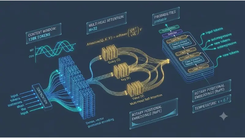
The core operation of a Transformer is Scaled Dot-Product Attention. Given input token embeddings, the network projects each token vector into three distinct spaces using learned linear projections: Query (Q), Key (K), and Value (V):
$$\text{Attention}(Q, K, V) = \text{softmax}\left( \frac{QK^T}{\sqrt{d_k}} \right) V$$
The dot product QKT measures similarity scores between every pair of tokens. The scaling factor 1 / √(dk) (where dk is the key vector dimension) prevents dot product magnitudes from growing excessively large in high dimensions, which would push the softmax function into regions with near-zero gradients.
2. Multi-Head Attention (MHA) & Efficient Variants
Instead of computing attention once, Multi-Head Attention projects Queries, Keys, and Values into h separate subspace representations, allowing the model to simultaneously attend to information from different representation aspects (e.g., syntactic structure vs. semantic coreference) at different positions:
$$\text{MultiHead}(Q, K, V) = \text{Concat}(\text{head}_1, \dots, \text{head}_h) W^O$$
As LLM context windows expanded (e.g., to 128k+ tokens), standard MHA created severe memory bottlenecks during KV-cache generation. Modern LLMs use computational memory variations:
- Multi-Query Attention (MQA): Shares a single Key and Value head across all Query heads to drastically reduce KV-cache VRAM usage during inference.
- Grouped-Query Attention (GQA): Group Query heads into sub-clusters (e.g., LLaMA-3), balancing MQA efficiency with MHA quality.
3. Positional Encodings: From Sinusoidal to RoPE
Because self-attention is permutation-equivariant (it treats input sequences as an unordered set of tokens), positional information must be explicitly injected. Standard Transformers use absolute sinusoidal positional encodings:
$$PE_{(pos, 2i)} = \sin\left(\frac{pos}{10000^{2i/d_{\text{model}}}}\right), \quad PE_{(pos, 2i+1)} = \cos\left(\frac{pos}{10000^{2i/d_{\text{model}}}}\right)$$
Modern decoder-only LLMs prefer Rotary Position Embeddings (RoPE). RoPE rotates Query and Key vector representations in 2D complex space by an angle proportional to token position, naturally incorporating relative token distance directly into the inner product score:
$$R_{\Theta, m}^d R_{\Theta, n}^d = R_{\Theta, m-n}^d$$
4. Python Implementation: Scaled Dot-Product Attention from Scratch
import torch

import torch.nn as nn

import torch.nn.functional as F

import math


class ScaledDotProductAttention(nn.Module):

    """

    Computes Scaled Dot-Product Attention with optional causal masking.

    """

    def __init__(self, d_k: int):

        super().__init__()

        self.scale = 1.0 / math.sqrt(d_k)


    def forward(

        self,

        q: torch.Tensor, # [batch, heads, seq_len, d_k]

        k: torch.Tensor, # [batch, heads, seq_len, d_k]

        v: torch.Tensor, # [batch, heads, seq_len, d_v]

        mask: torch.Tensor = None # Causal mask for autoregressive decoding

    ) -> tuple[torch.Tensor, torch.Tensor]:

        # Compute raw attention scores Q * K^T

        scores = torch.matmul(q, k.transpose(-2, -1)) * self.scale


        if mask is not None:

            # Fill masked positions with negative infinity to zero them out in softmax

            scores = scores.masked_fill(mask == 0, float('-inf'))


        # Apply softmax to obtain normalized attention weights

        attn_weights = F.softmax(scores, dim=-1)


        # Multiply attention weights by Value vectors

        output = torch.matmul(attn_weights, v)

        return output, attn_weights


# Example Execution

batch_size, num_heads, seq_len, d_k = 2, 4, 8, 64

q_vec = torch.randn(batch_size, num_heads, seq_len, d_k)

k_vec = torch.randn(batch_size, num_heads, seq_len, d_k)

v_vec = torch.randn(batch_size, num_heads, seq_len, d_k)


# Create lower-triangular causal mask for autoregressive prediction

causal_mask = torch.tril(torch.ones(seq_len, seq_len)).unsqueeze(0).unsqueeze(0)


attention_layer = ScaledDotProductAttention(d_k)

context_output, weights = attention_layer(q_vec, k_vec, v_vec, mask=causal_mask)

print("Attention Output Matrix Shape:", context_output.shape)

print("Attention Weights Matrix Shape:", weights.shape)
Interactive Quick Review: Encoder-Decoder vs. Decoder-Only Models
Why have decoder-only architectures (e.g., GPT-4, LLaMA) superseded encoder-decoder models (e.g., T5) as the dominant paradigm for general-purpose LLMs?
Toggle Answer
Answer: Decoder-only models unify all NLP tasks (summarization, translation, code generation, reasoning) into a single autoregressive sequence-to-sequence completion objective. They scale more efficiently with compute and memory during pre-training, naturally supporting few-shot and zero-shot in-context learning without requiring task-specific head adaptation.
Taxonomy & Optimization Comparison Matrix
| Architecture Family | Attention Mechanism | Primary Training Objective | Representative Models | Best Suited Tasks |
|---|---|---|---|---|
| Encoder-Only | Bidirectional Self-Attention | Masked Language Modeling (MLM) | BERT, RoBERTa, DeBERTa | Classification, Named Entity Recognition, Sentence Embeddings |
| Decoder-Only | Causal (Masked) Self-Attention | Autoregressive Next-Token Prediction | GPT-4, LLaMA-3, Mistral, Claude | Open-ended Text Generation, Reasoning, Code Synthesis, In-Context Learning |
| Encoder-Decoder | Cross-Attention + Causal Attention | Span Masking / Sequence-to-Sequence Loss | T5, BART, Whisper | Machine Translation, Text Summarization, Audio Transcription |
| Sparse Mixture-of-Experts (MoE) | Routed Top-K Self-Attention | Autoregressive MoE Router Loss | Mixtral 8x7B, Grok-1, DeepSeek-V2 | Ultra-high-capacity inference with reduced active parameter compute cost |
Applications, Trade-offs, & Future Outlook
Real-World Applications
- Enterprise Knowledge Synthesis: Powering organizational copilot systems to parse, summarize, and execute operations over internal document repositories.
- Automated Software Engineering: Generating, refactoring, and debugging code across complex multi-file software engineering pipelines.
- Multimodal Reasoning Systems: Unifying textual sequence modeling with vision, speech, and structured database operations in unified Transformer decoders.
Engineering Trade-offs
The core bottleneck of Transformers is Quadratic Attention Complexity: standard self-attention requires O(N2) compute and memory scaling relative to sequence length N. While flash attention algorithms (e.g., FlashAttention-3) optimize GPU SRAM memory tiling to avoid materializing full N × N matrices, ultra-long contexts still demand vast amounts of VRAM for KV-cache retention during batch inference.
Future Outlook & Emerging Research
Research is advancing along two main fronts: Sub-Quadratic Hybrid Architectures—such as State Space Models (Mamba) and linear attention models that achieve O(N) linear memory scaling—and Test-Time Compute Scaling (e.g., OpenAI o1/o3 paradigms), which spend additional reasoning compute budget during inference via Monte Carlo tree search and chain-of-thought verification loops.
Frequently Asked Questions
What is the KV-Cache in LLM Inference?
The KV-cache stores pre-computed Key and Value vector representations for previous tokens in the context window during autoregressive text generation. This prevents recomputing past token vectors at every new token generation step, speeding up generation from O(N2) to O(N) compute per step at the cost of higher VRAM usage.
How does Grouped-Query Attention (GQA) reduce VRAM requirements?
GQA divides Query heads into groups that share a single Key and Value head. For example, an 8:1 GQA ratio reduces the memory footprint of stored KV-cache vectors by 8× compared to standard Multi-Head Attention, enabling larger batch sizes and longer context windows on edge GPUs.
What is the difference between Pre-LayerNorm and Post-LayerNorm?
Post-LayerNorm applies normalization after the residual connection addition, which can cause exploding or vanishing gradients in very deep Transformer networks without careful learning rate warmups. Pre-LayerNorm applies normalization directly to the inputs of attention and feed-forward sub-layers before the residual connection, stabilizing gradient flow during large-scale pre-training.
How does Mixture-of-Experts (MoE) scale LLM model capacity?
MoE replaces dense Feed-Forward Networks (FFN) with multiple parallel “expert” networks. A learned router dynamically routes each token to the top 1 or 2 most relevant experts. This allows a model to possess 47B+ total parameters while activating only ~13B parameters per token, lowering computational cost per inference step.
End-of-Page Exercises & Assessment
Part 1: Review Questions
Q1: Define the mathematical role of the Query, Key, and Value matrices in self-attention.
Answer: The Query matrix Q represents the current token searching for context; the Key matrix K represents candidate tokens offering context match labels; the Value matrix V contains the actual semantic feature vectors aggregated based on softmax-normalized similarity scores between Q and K.
Q2: Why is the scaling factor 1 / √(dk) necessary in Scaled Dot-Product Attention?
Answer: For large vector dimensions dk, dot products grow large in magnitude, pushing the softmax function into regions with extremely small gradients (vanishing gradient problem). Dividing by √(dk) maintains variance near 1.0, preserving healthy gradient flow.
Q3: State the core mathematical advantage of Rotary Position Embeddings (RoPE).
Answer: RoPE encodes positional information by rotating Query and Key vectors in complex space. The inner product ⟨RΘ,m q, RΘ,n k⟩ depends purely on the relative distance (m – n) between token positions rather than their absolute positions.
Q4: What is Causal Masking in Decoder-Only LLMs?
Answer: Causal masking sets attention score elements above the main diagonal to -∞ before applying softmax. This prevents the model from looking ahead at future tokens during autoregressive training and generation.
Q5: What is SwiGLU and why is it preferred over ReLU in modern FFN blocks?
Answer: SwiGLU (Swish Gated Linear Unit) combines the Swish activation function with a gating mechanism. It provides smoother gradient propagation and empirically improves task accuracy compared to standard ReLU activations in architectures like LLaMA.
Part 2: Thought-Provoking Questions
Q1: Memory Wall in Long-Context Inference
Scenario: An engineering team attempts to serve a 70B parameter LLM with a 128k context window using standard Multi-Head Attention. While GPU compute utilization is low, the server runs out of VRAM (OOM error) after serving just 2 concurrent user requests.
Analysis: The memory failure is caused by the KV-cache footprint scaling linearly with batch size and context length under MHA. At 128k tokens, the FP16 KV-cache for a single sequence in a 70B model requires tens of gigabytes of VRAM. Mitigating this requires converting the model to Grouped-Query Attention (GQA), applying PagedAttention (vLLM) to eliminate memory fragmentation, and quantizing stored KV-cache entries to 4-bit or 8-bit precision.
Q2: Attention Saturation and “Needle in a Haystack” Failure
Scenario: A 1M context LLM correctly retrieves a specific sentence hidden in a 10k token prompt, but fails to retrieve the exact same sentence when buried in the middle of a 100k token prompt.
Analysis: This is an example of the “Lost in the Middle” phenomena and attention degradation. As context length grows, the softmax distribution spreads probability density across thousands of tokens, smoothing out sharpness on relevant key-query matches. Mitigating this requires training with explicit long-context synthetic datasets, adjusting RoPE base frequencies (θ scaling), and employing attention temperature recalibration.
Part 3: Numerical Engineering Problems
Problem 1: Self-Attention Matrix Parameter and FLOP Count
Question: Consider a Transformer layer with hidden dimension dmodel = 4096 and key/value projection dimension dk = dv = dmodel.
1. Calculate the total parameter count across all four linear projection matrices (WQ, WK, WV, WO) in a standard Multi-Head Attention block (ignoring bias terms).
2. For an input sequence length N = 2048 tokens, compute the FLOP count required to evaluate the raw dot product matrix Q · KT for a single sequence sample (assume 2 FLOPs per multiply-accumulate operation).
Step-by-step Solution:
1. Parameter Count Calculation:
• Each projection matrix (WQ, WK, WV, WO) has shape [dmodel, dmodel] = [4096, 4096].
• Parameters per matrix = 4096 × 4096 = 16,777,216 (16.78M).
• Total parameters for 4 matrices = 4 × 16,777,216 = 67,108,864 parameters (~67.1M).
2. Attention Dot-Product FLOP Count Calculation:
• Matrix Q has shape [N, dmodel] = [2048, 4096].
• Matrix KT has shape [dmodel, N] = [4096, 2048].
• Matrix multiplication [2048, 4096] × [4096, 2048] requires 2 × N × N × dmodel FLOPs.
• FLOPs = 2 × 2048 × 2048 × 4096 = 2 × 4,194,304 × 4096 = 34,359,738,368 FLOPs (~34.36 GFLOPs).
Final Answer: Total attention projection parameters = 67,108,864 (~67.1M). Attention score matrix multiplication requires 34,359,738,368 FLOPs (~34.36 GFLOPs).
Problem 2: KV-Cache VRAM Footprint Calculation
Question: A deployment server hosts a 32-layer LLM with 32 Query heads, 8 Key/Value heads (Grouped-Query Attention), head dimension dhead = 128, sequence context length N = 8192 tokens, and batch size B = 16 sequences.
If Key and Value vectors are stored in FP16 precision (2 bytes per element), calculate the total VRAM required in Megabytes (MB) to store the KV-cache during inference.
Step-by-step Solution:
1. Determine elements per token per layer:
• Key elements per token = num_kv_heads × dhead = 8 × 128 = 1024.
• Value elements per token = num_kv_heads × dhead = 8 × 128 = 1024.
• Total elements per token per layer = 1024 + 1024 = 2048 elements.
2. Compute elements across all layers, context length, and batch size:
• Total elements = B × L × N × 2048
• Total elements = 16 × 32 × 8192 × 2048 = 512 × 8192 × 2048 = 8,589,934,592 elements.
3. Convert elements to Bytes and Megabytes (1 MB = 1,048,576 Bytes):
• Total Bytes (FP16) = 8,589,934,592 × 2 Bytes = 17,179,869,184 Bytes.
• Total MB = 17,179,869,184 / (1024 × 1024) = 16,384 MB (16 GB).
Final Answer: The total KV-cache VRAM memory footprint is 16,384 MB (16.0 GB).
Natural Language Processing & GenAI Sub-Cluster
-
Generative AI, Prompt Engineering & RAG
Master in-context zero/few-shot learning, instruction tuning, vector retrieval grounding, and RAG architectures. -
AI Agents & Autonomous Workflows
Explore ReAct agent loops, multi-agent orchestration, tool use, memory systems, and agent frameworks. -
Vector Databases & Semantic Search
Dive into dense embedding models, HNSW/IVF vector indexing, distance metrics, and hybrid search systems. -
Natural Language Processing Hub
Return to the main Natural Language Processing overview covering text preprocessing, tokenization, embeddings, and language models.
External Academic & Technical References
- Attention Is All You Need (Vaswani et al., NeurIPS 2017) – The seminal paper introducing the Transformer architecture and Multi-Head Self-Attention.
- RoFormer: Enhanced Transformer with Rotary Position Embedding (Su et al., 2021) – Key paper deriving Rotary Position Embeddings (RoPE) for relative sequence position encoding.
- GQA: Training Generalized Multi-Query Transformer Models from Multi-Head Checkpoints (Ainslie et al., 2023) – Foundational research on Grouped-Query Attention for high-throughput LLM inference.